1M rides a day. What do you do in the first 5 minutes?
Requirements in depth: functional vs non-functional, SLIs, SLOs and error budgets, nines arithmetic, capacity estimation and how the numbers pick the design.
 Video · 60 secondsWatch the short versionSame diagrams and numbers. Tap to play.
In this lesson you will learn
- How to write functional requirements as things a user does
- How to turn "fast" and "reliable" into measurable targets (SLOs and error budgets)
- How to estimate from daily users to peak requests, storage and servers
- What to put in and out of scope in the first 5 minutes
Builds on Lesson 1: What system design is 18 min read + 60 s video Next: Performance vs scalability, measured
Drafted with AI assistance, then checked and edited by a human engineer · How we write
Short answer
Write functional requirements as user actions and non-functional ones as SLOs: an SLI (good ÷ valid events), a target and a window. 99.9% over 30 days leaves a 43.2 minute error budget. Estimate daily events to peak rate to storage to nodes. For a ride app, 25,000 location writes a second against 35 new rides picks an in-memory geo index for location and idempotent, strongly consistent payments.
| SLO | SLI (good ÷ valid events) + target + window, e.g. 99% of matches under 5 s over 30 days |
|---|---|
| Error budget | (1 − SLO) × window: 99.9% over 30 days = 43.2 min, 99.99% = 4.32 min |
| Availability maths | Serial: multiply; parallel: 1 − (1 − A)^n, only if failures are independent |
| Peak location load | 100,000 online drivers ÷ 4 s = 25,000 writes/s (assumed figures) |
| Peak booking load | 1M rides ÷ 86,400 s × 3 ≈ 35 new rides/s, about 720 times less |
| Location store | Latest position only, about 10 MB, overwritten, TTL, geohash or H3 cells |
| Payments | Idempotency key + strongly consistent database, never a TTL cache |
A design is checked against its requirements, and "fast and reliable" cannot be measured, so it cannot decide anything. Requirements turn into indicators, targets, budgets and capacity numbers, and those numbers choose the storage, the consistency model and the node count. Interview question: "Design a ride app for one million rides a day. What do you pin down before you draw?"
Prerequisites
Rates per second. A server's load is measured in requests per second. A day has 24 × 60 × 60 = 86,400 seconds, so any daily count divided by 86,400 is its average rate: 1 million a day is 11.6 a second.
Peak versus average. The busiest window divided by the average is the peak factor, and capacity is sized for the peak plus headroom. The article on performance vs scalability for a ticket rush covers how a load balancer and a waiting room absorb a burst.
Percentiles. The mean hides the slow tail, so latency targets are percentiles: p99 is the value that 99% of measurements are at or below.
Definitions
Functional requirement: a behaviour the system must provide, stated as an observable action and its result. It is true or false for a given build.
Non-functional requirement (NFR): a quality the system must have while doing that (latency, availability, freshness, durability, correctness under retry). It is a matter of degree, so it needs a number, a measurement point and a window.
SLI (service level indicator): a measured ratio of good events to valid events, for example "match requests answered within 5 s ÷ all valid match requests", taken at a stated point such as the load balancer.
SLO (service level objective): an internal target for an SLI over a window, such as 99% over a rolling 30 days. SLA (service level agreement): a customer contract with a looser target and a penalty, such as service credits.
Error budget: the amount of failure an SLO permits, (1 − SLO) × window, counted in minutes or in failed requests. Overspending it moves priority from features to reliability.
Geospatial index: a structure that maps positions to cell ids so "drivers near this point" reads a few cells, not every driver.
Idempotency: an operation applied twice has the same effect as applied once. Payment APIs use an idempotency key: a unique id the client sends so the server recognises a retry.
How it works: from questions to numbers
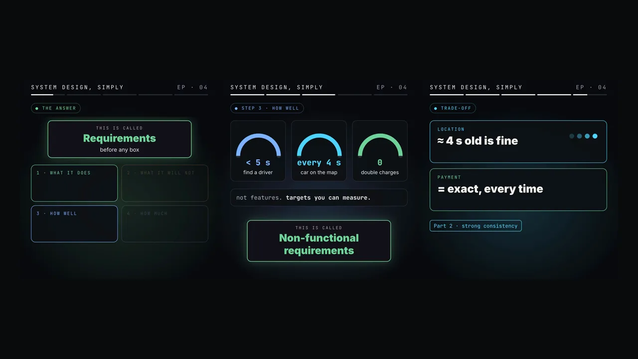
Requirements work has four outputs, and each feeds a later decision. Functional requirements decide which components exist, scope which ones are left out, non-functional requirements how each is built (storage engine, replication mode, cache policy), and estimates how many you run and which one gets the deep dive.
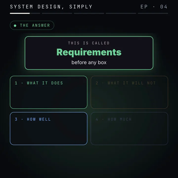
Functional vs non-functional. A functional requirement can be checked with one request in a test environment. A non-functional one can only be checked statistically, over many requests and time. Break a functional requirement and a feature is missing; break a non-functional one and the feature exists but is too slow, wrong under retry or down at the busiest hour. Late NFRs cause most redesigns, because they can change the type of store as well as the endpoints.
Write functional requirements as actions with outcomes, including the failure outcome. "Rider requests a ride" is incomplete. "Rider requests a ride and, within the match SLO, either gets a driver or is told none is available" defines a timeout, a terminal state and something an SLI can count. "Rider pays" becomes "exactly once, even if the app retries".

Scope with reasons. Ratings and chat do not touch the request, match, track, pay path. Scheduled rides need a durable timer service and supply planning, a separate design. Stating the reason invites an objection early, while changing scope is still cheap.
The question checklist. Ask only the questions whose answers would change a component:
- Actors and actions: who calls the system, and which three to five actions matter?
- Scale and shape: events per day, peak factor, growth per year, one region or many?
- Latency: which action has a deadline, at which percentile, measured where?
- Freshness: how old may displayed data be? This sets cache TTLs and acceptable replication lag.
- Correctness: what must never be lost, doubled or reordered (money, seats, stock)?
- Availability and degradation: downtime per month, and which partial outage is acceptable?
- Read/write ratio: mostly read, mostly written, or both?
- Retention and compliance: what is kept, how long, who may see it?
- Background load: does anything send data while nobody is using the product, such as idle drivers?
SLIs, SLOs, SLAs and error budgets
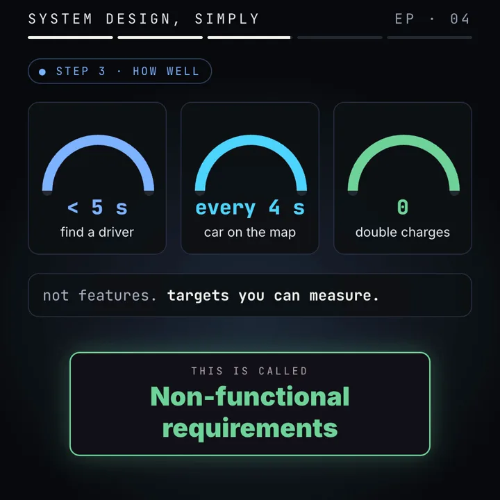
An NFR becomes operational when it has four parts: what is counted (the SLI), where it is measured, the target and the window. The Google SRE workbook recommends SLIs as good events ÷ valid events, so every SLI sits between 0% and 100%.
| NFR as spoken | SLI (good ÷ valid) | Measured at | SLO (assumed) |
|---|---|---|---|
| Find a driver quickly | matches answered (driver or "none available") within 5 s ÷ valid requests | API gateway | 99% over 30 days |
| Car moves smoothly on the map | renders showing a position at most 8 s old ÷ all renders | rider app, sampled | 99% over 30 days |
| Booking is up | bookings without a server error ÷ valid bookings | load balancer | 99.9% over 30 days |
| Never charge twice | rides with exactly one capture ÷ paid rides | ledger, daily | 100%: an invariant, no budget |
Valid excludes requests the system should reject (malformed input, a client cancelling), or a bad client burns your budget. The measurement point decides what is visible: a server timer misses DNS, TLS and mobile network time; a client timer includes them but is noisy. The freshness target is 8 s, two update intervals, because jitter or one lost packet would break a 4 s target constantly. "Send every 4 s" is an input; the SLO measures what the rider sees.
Percentiles and the tail. If one action fans out to n parallel backend calls, each slow 1% of the time, it is slow whenever any call is: P(slow) = 1 − 0.99n. For n = 10 that is 9.6%, for n = 100 it is 63.4%. So a component inside the match path needs a tighter target (p99.9) than the user-facing SLO (p99).
Error budget arithmetic. A 30-day window is 30 × 24 × 60 = 43,200 minutes. The budget is (1 − SLO) × 43,200:
SLO        budget per 30 days            budget per 365 days
99%        0.01 × 43,200 = 432 min (7.2 h)      0.01 × 8,760 h = 87.6 h (3.65 days)
99.9%      0.001 × 43,200 = 43.2 min            0.001 × 8,760 h = 8.76 h
99.95%     0.0005 × 43,200 = 21.6 min           0.0005 × 8,760 h = 4.38 h
99.99%     0.0001 × 43,200 = 4.32 min           0.0001 × 525,600 min = 52.56 min
99.999%    0.00001 × 43,200 = 0.432 min (25.9 s) 0.00001 × 525,600 min = 5.26 min
Request-based budgets track user impact more closely, because 10 minutes down at 3 a.m. and at the evening peak are not equally bad: 30 days × 1,000,000 = 30,000,000 bookings, and 99.9% permits 0.001 × 30,000,000 = 30,000 failures. An error budget policy states what happens when it runs out, typically a freeze on risky releases.
Burn rate is spend relative to plan: 1 uses the budget in exactly 30 days. Spending 2% of it in one hour is 0.02 × 720 h = 14.4, which empties the budget in 720 ÷ 14.4 = 50 hours. Alerting on burn rate keeps pages proportional to user harm.
Availability of a chain. Components in series must all be up, so availabilities multiply. Gateway 99.99%, matcher 99.95% and database 99.99% give 0.9999 × 0.9995 × 0.9999 ≈ 99.93%, which is lower than the weakest part. Redundant copies in parallel fail only if all fail: 1 − (1 − A)n, so two 99.9% replicas give 1 − 0.0012 = 99.9999%. That assumes independent failures; replicas sharing a power feed, a deploy pipeline or a config fail together, close to a single copy. Each added nine allows ten times less downtime and costs redundancy and slower releases, so pick the target from user need; the SRE book's "Embracing Risk" chapter argues this in detail.
Capacity estimation, step by step
Estimation is a pipeline of single multiplications or divisions, with each assumption labelled:
- Actors to events. DAU (daily active users) × actions per user = events per day. Here rides per day are given; the hidden events are location updates.
- Events to average rate. Events per day ÷ 86,400.
- Average to peak. × peak factor (3 assumed).
- Concurrency. Little's law: L = λ × W. Rides in progress = ride arrival rate × ride duration. This turns rates into open connections and memory.
- Storage. Rate × bytes per record × retention × replicas.
- Bandwidth. Peak rate × bytes on the wire (payload plus headers).
- Nodes. ceil(peak demand ÷ (per-node capacity × target utilisation)) + 1 spare. Per-node capacity comes from a load test.
Why a target utilisation of about 50%. In the simplest queueing model (M/M/1) the queue wait is ρ ÷ (1 − ρ) service times at utilisation ρ: 1 at 0.5, 4 at 0.8, 9 at 0.9. 50% leaves room for a higher peak and a failed node.
Reference latencies. From the widely cited latency table (see the sources): a memory reference is about 100 ns, a random 4 KB SSD read 150 µs, a round trip inside one data centre 500 µs, a disk seek 10 ms, California to the Netherlands and back 150 ms. So an in-memory store is limited by round trips and request handling, not the write itself. 25,000 writes a second, each waiting for its own 0.5 ms round trip in turn, needs 25,000 × 0.5 ms = 12.5 s of waiting per second: use at least 13 concurrent connections, or pipeline 100 commands per round trip for 250 round trips a second.
See the ticket rush article on load balancing for spreading connections over gateway nodes, and why that fixes scalability rather than performance.
How the location load shapes the design
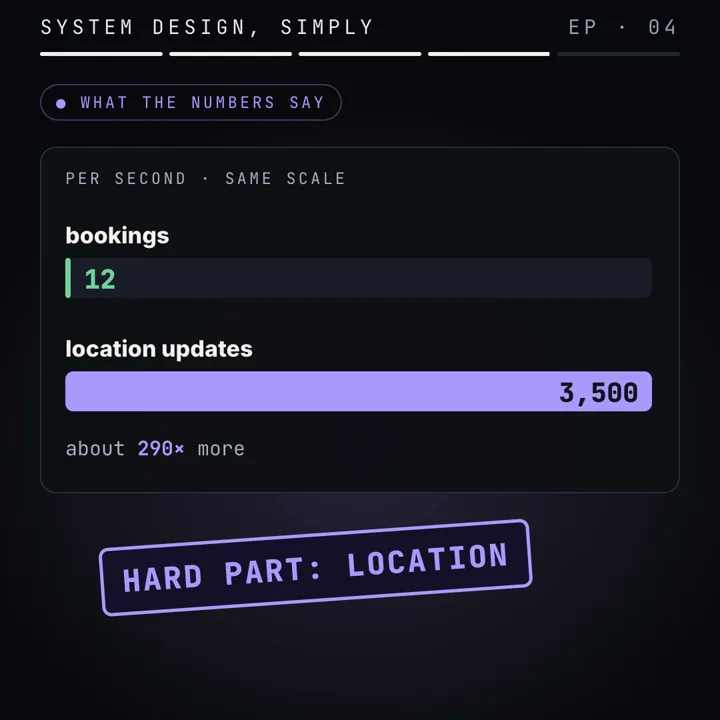
Read/write ratio picks the architecture. A read-heavy system is solved with caches and replicas: write once, serve many copies. A write-heavy one cannot be cached out of trouble; every write must land. The feed in fan-out on read vs fan-out on write is read-heavy. Location is the opposite: every online driver writes every 4 s, a watching rider reads about one update per update, and the matcher searches about 35 times a second. Most written values are never read before a newer one replaces them.
Split current position from history. They have opposite requirements:
- Latest location: one value per driver, overwritten, useful for seconds. 100,000 drivers × 100 B ≈ 10 MB. The size is small and the rate is the problem, so it goes in an in-memory store such as Redis.
- Trail history: append-only, rides only, for receipts and disputes. About 30 GB a day, written in batches to a log or write-optimised table.
TTL as a liveness signal. Store each driver's latest position with an expiry, for example 30 s (assumed, about seven missed updates). A phone that loses signal drops out of search by itself. Redis caveat: a geo index is one sorted set and expiry applies to whole keys, not members. So use a per-driver key with a TTL plus a sweep of the geo set by last-seen time, or one geo key per cell per short time bucket, so buckets expire whole.
Write coalescing and batching. Coalescing drops superseded values of one key: a phone that reconnects and flushes ten buffered points needs only the newest in the latest store. Batching groups many values into one write: buffering each ride's trail for 60 s turns 15 writes into one, so 10,417 points a second at peak become about 694 writes. A crash can lose up to 60 s of trail, fine if the fare comes from a durable event at ride end.
Geospatial indexing. "Drivers within 2 km" over 100,000 points is a scan unless positions are bucketed:
- Geohash interleaves longitude and latitude bits and encodes 5 bits per base-32 character. A 6-character geohash is 30 bits, 15 for longitude and 15 for latitude: 360° ÷ 215 by 180° ÷ 215, about 1.22 km by 0.61 km at the equator. Points either side of a cell edge may share no prefix, so a search includes the 8 neighbours. Redis stores a geo index as a sorted set scored by a 52-bit geohash and scans the 1 + 8 cell ranges covering the shape (GEOADD, O(log N) per member; GEOSEARCH, O(N + log M)).
- H3 covers the Earth with hexagons at 16 resolutions. Resolution 8 cells average 0.737 km², an edge of about 0.53 km. All six neighbours sit at the same centre distance, so a cell plus one ring (7 cells, about 5.2 km²) is a near-circular search area; k rings hold 3k(k + 1) + 1 cells.
The match radius picks the cell size: 1 to 3 km in a city points at geohash length 6 or H3 resolution 7 to 8, so a search reads a handful of cells instead of the whole fleet.
Consistency per data type
Set consistency for each kind of data rather than for the whole system, so data that tolerates staleness can stay on the cheap path.
| Data | Requirement | Consequence |
|---|---|---|
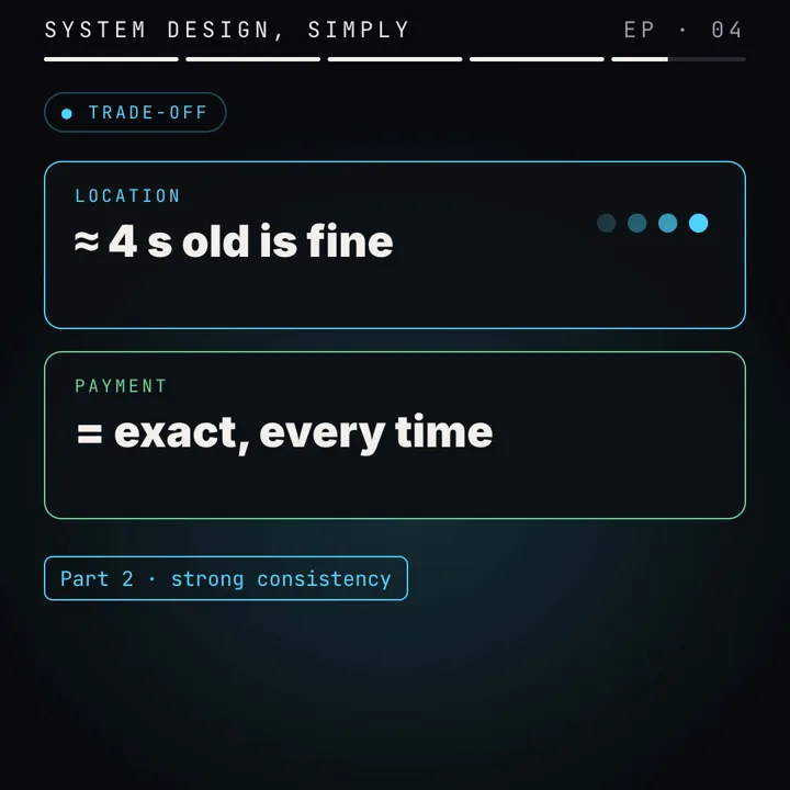
| Driver position | Stale-tolerant: 8 s old or one lost update is fine | In memory, last write wins, asynchronous replication, TTL |
| Ride state (requested, accepted, finished) | One driver per ride; transitions in order | Conditional update, as for one seat |
| Payment | Exactly once, durable, auditable | Idempotency key, strongly consistent store, append-only ledger |
| Trail history | Durable eventually; minutes of delay fine | Batched appends to a log or table |
If an offer reaches two drivers, acceptance is the same race as a seat sale: one conditional update that checks and sets in one statement, explained in how an atomic update stops two fans buying one seat.
Payments add retries: a client that times out cannot know whether the charge happened. It sends one unique key per payment attempt with every retry; the server stores the key with the result and answers a repeat with the stored result. Stripe's API documentation on idempotent requests describes this contract. Write the key in the same transaction as the charge, or a crash between them reopens the double charge.
Worked example
The video's scenario: a ride app in one country, and a large venue emptying at night into a sharp peak. Scope: request, match, track, pay. Given: 1,000,000 rides a day; everything else is assumed and labelled.
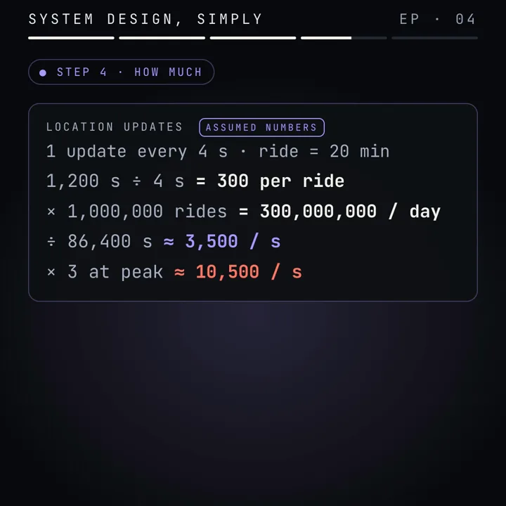
GIVEN    rides per day                        1,000,000
ASSUMED  ride length                          20 min = 1,200 s
ASSUMED  location interval                    4 s
ASSUMED  peak factor                          3
ASSUMED  drivers online at peak               100,000 (on a ride or idle)

RIDES      1,000,000 ÷ 86,400                 ≈ 11.6/s avg, × 3 ≈ 34.7/s peak
TRAIL      1,200 s ÷ 4 s = 300 points a ride; × 1,000,000 = 300,000,000 a day
           300,000,000 ÷ 86,400               ≈ 3,472/s avg, × 3 ≈ 10,417/s peak
IN RIDE    Little's law: 11.6/s × 1,200 s     ≈ 13,889 avg, × 3 ≈ 41,667 peak
           check: 41,667 ÷ 4 s                ≈ 10,417/s (matches TRAIL peak)
ALL GPS    100,000 drivers ÷ 4 s              = 25,000 writes/s at peak
           25,000 ÷ 34.7                      ≈ 720 location writes per new ride
LATEST     100,000 × 100 B (assumed per row)  = 10 MB in memory
HISTORY    300,000,000 × 100 B                = 30 GB a day
           (30 GB + 1 GB of 1 KB ride records, assumed) × 365 × 3 replicas ≈ 33.9 TB a year
INGRESS    25,000 × 200 B × 8 bits            = 40 Mbit/s at peak
SOCKETS    41,667 rides × 2 phones + 58,333 idle drivers ≈ 141,667 open
NODES      store:   25,000 ÷ (10,000 × 0.5) = 5, + 1 spare = 6   (10,000/s per node assumed)
           gateway: 141,667 ÷ (50,000 × 0.5) = 5.7 → 6, + 1 = 7 (50,000 sockets per node assumed)
BUDGET     booking SLO 99.9% over 30 days     = 43.2 min, or 30,000 failed bookings
Booking is about 35 writes a second, easy for one relational database. Location is 25,000 writes a second of data worthless after seconds. Bandwidth is trivial at 40 Mbit/s; the difficulty is the number of writes and sockets, so the deep dive goes to location.
Code
The calculator behind every number above: assumptions in one dictionary, the article's formulas as functions. Plain Python 3, no libraries.
# Requirements calculator for a ride app: load, storage, servers, SLO budgets.
# Every value in ASSUMED is a guess you say out loud and invite correction on.
# Plain Python 3, no libraries. Change one value, run again, watch what moves.
import math

ASSUMED = {
    "rides_per_day": 1_000_000,     # given by the interviewer
    "ride_minutes": 20,             # assumed average ride length
    "update_every_s": 4,            # assumed: driver phone sends GPS every 4 s
    "peak_factor": 3,               # assumed: busiest hour is 3x the average
    "online_drivers_peak": 100_000, # assumed: drivers online at peak, on a ride or idle
    "bytes_per_update": 100,        # assumed: stored row incl. index overhead
    "wire_bytes_per_update": 200,   # assumed: same update plus protocol headers
    "bytes_per_ride": 1_000,        # assumed: one ride record
    "replicas": 3,                  # assumed: copies of every stored byte
    "writes_per_node": 10_000,      # assumed: measured by a load test, one store node
    "conns_per_node": 50_000,       # assumed: open WebSockets one gateway node holds
    "target_util": 0.5,             # plan nodes at 50% so queues stay short
    "trail_batch_s": 60,            # history buffered per ride and flushed every 60 s
}
DAY = 24 * 60 * 60                  # 86,400 s
MONTH_MIN = 30 * 24 * 60            # 43,200 min in a 30-day window


def load(a):
    per_ride = a["ride_minutes"] * 60 / a["update_every_s"]
    rides_s = a["rides_per_day"] / DAY
    on_ride_peak = rides_s * a["ride_minutes"] * 60 * a["peak_factor"]   # Little's law x peak
    loc_peak = a["online_drivers_peak"] / a["update_every_s"]           # every online driver
    trail_s = rides_s * per_ride
    return {
        "updates per ride": per_ride,
        "trail updates per day": a["rides_per_day"] * per_ride,
        "trail updates/s (avg)": trail_s,
        "trail updates/s (peak)": trail_s * a["peak_factor"],
        "new rides/s (avg)": rides_s,
        "new rides/s (peak)": rides_s * a["peak_factor"],
        "rides in progress (peak)": on_ride_peak,
        "all location writes/s (peak)": loc_peak,
        "location writes per new ride (peak)": loc_peak / (rides_s * a["peak_factor"]),
        "latest-location store MB": a["online_drivers_peak"] * a["bytes_per_update"] / 1e6,
        "history GB per day": a["rides_per_day"] * per_ride * a["bytes_per_update"] / 1e9,
        "stored TB per year (replicas)": (a["rides_per_day"] * (per_ride * a["bytes_per_update"]
                                          + a["bytes_per_ride"])) * 365 * a["replicas"] / 1e12,
        "history writes/s batched (peak)": trail_s * a["peak_factor"] / (a["trail_batch_s"] / a["update_every_s"]),
        "ingress Mbit/s (peak)": loc_peak * a["wire_bytes_per_update"] * 8 / 1e6,
        "open connections (peak)": 2 * on_ride_peak + (a["online_drivers_peak"] - on_ride_peak),
    }


def nodes(demand, per_node, util):
    # N for the load, +1 so one node can fail at peak (N+1)
    return math.ceil(demand / (per_node * util)) + 1


def budget_minutes(slo, window_min=MONTH_MIN):
    return (1 - slo) * window_min


def serial(*parts):            # every part must be up
    return math.prod(parts)


def parallel(a, n):            # any one of n independent copies is enough
    return 1 - (1 - a) ** n


def p_some_slow(n, p_fast=0.99):  # one request fans out to n backends
    return 1 - p_fast ** n


def geohash_cell_m(length):    # cell size at the equator
    bits = 5 * length
    lon_bits, lat_bits = (bits + 1) // 2, bits // 2
    m_per_deg = 111_320
    return 360 / 2 ** lon_bits * m_per_deg, 180 / 2 ** lat_bits * m_per_deg


if __name__ == "__main__":
    a = ASSUMED
    out = load(a)
    for k, v in out.items():
        print(f"{k:<38}{v:>16,.1f}")
    print(f"{'store nodes (peak writes, N+1)':<38}"
          f"{nodes(out['all location writes/s (peak)'], a['writes_per_node'], a['target_util']):>16}")
    print(f"{'gateway nodes (connections, N+1)':<38}"
          f"{nodes(out['open connections (peak)'], a['conns_per_node'], a['target_util']):>16}")
    for slo in (0.99, 0.999, 0.9995, 0.9999, 0.99999):
        print(f"{'error budget min, 30 days, %.3f%%' % (slo * 100):<38}{budget_minutes(slo):>16,.2f}")
    print(f"{'failed bookings allowed at 99.9%':<38}{(1 - 0.999) * a['rides_per_day'] * 30:>16,.0f}")
    print(f"{'serial 99.99 x 99.95 x 99.99 %':<38}{serial(0.9999, 0.9995, 0.9999) * 100:>16.4f}")
    print(f"{'two parallel copies of 99.9 %':<38}{parallel(0.999, 2) * 100:>16.4f}")
    for n in (1, 10, 100):
        print(f"{'P(slow) fan-out to %d at p99' % n:<38}{p_some_slow(n) * 100:>15.1f}%")
    for n in (5, 6, 7):
        w, h = geohash_cell_m(n)
        print(f"{'geohash length %d cell, m' % n:<38}{w:>8,.0f} x {h:>6,.0f}")
Real output of python3 estimate.py:
updates per ride                                 300.0
trail updates per day                    300,000,000.0
trail updates/s (avg)                          3,472.2
trail updates/s (peak)                        10,416.7
new rides/s (avg)                                 11.6
new rides/s (peak)                                34.7
rides in progress (peak)                      41,666.7
all location writes/s (peak)                  25,000.0
location writes per new ride (peak)              720.0
latest-location store MB                          10.0
history GB per day                                30.0
stored TB per year (replicas)                     33.9
history writes/s batched (peak)                  694.4
ingress Mbit/s (peak)                             40.0
open connections (peak)                      141,666.7
store nodes (peak writes, N+1)                       6
gateway nodes (connections, N+1)                     7
error budget min, 30 days, 99.000%              432.00
error budget min, 30 days, 99.900%               43.20
error budget min, 30 days, 99.950%               21.60
error budget min, 30 days, 99.990%                4.32
error budget min, 30 days, 99.999%                0.43
failed bookings allowed at 99.9%                30,000
serial 99.99 x 99.95 x 99.99 %                 99.9300
two parallel copies of 99.9 %                  99.9999
P(slow) fan-out to 1 at p99                       1.0%
P(slow) fan-out to 10 at p99                      9.6%
P(slow) fan-out to 100 at p99                    63.4%
geohash length 5 cell, m                 4,892 x  4,892
geohash length 6 cell, m                 1,223 x    611
geohash length 7 cell, m                   153 x    153
What to observe: set update_every_s to 2 and the location rates double (50,000 writes a second, store nodes 6 to 11) while new rides stay at 34.7 a second. Set target_util to 0.8 and both node counts fall to 5, paid for in queueing delay. online_drivers_peak moves the store more than rides_per_day does: idle drivers are the hidden load.
A requirements template to fill top to bottom:
REQUIREMENTS: <system>

1. FUNCTIONAL (3 to 5 actions, each with its failure outcome)
   - Rider requests a ride; gets a driver or "none available" within the match SLO
   - Driver accepts; exactly one driver per ride
   - Rider and driver see the car position
   - Rider pays exactly once, even when the app retries

2. OUT OF SCOPE (with reason)
   - Ratings, chat: not on the core path
   - Scheduled rides: needs a durable timer service, separate design

3. SLOs (SLI = good / valid, where measured, target, window)
   - Match: answered within 5 s / valid requests, at gateway, 99%, 30 days
   - Freshness: shown position at most 8 s old / renders, in app, 99%, 30 days
   - Booking availability: non-5xx / valid, at load balancer, 99.9%, 30 days
     budget 43.2 min or 30,000 failed bookings per 30 days
   - Payments: one capture per paid ride, invariant, daily reconciliation

4. ESTIMATES (assumptions labelled)
   - Given 1,000,000 rides/day; assumed 20 min, 4 s interval, peak x3, 100,000 online drivers
   - Rides 11.6/s avg, 34.7/s peak; location 25,000 writes/s peak
   - Latest store 10 MB; history 30 GB/day; 33.9 TB/year with 3 replicas
   - Sockets about 141,667; store 6 nodes, gateway 7 nodes (N+1, 50% utilisation)

5. CONSISTENCY PER DATA TYPE
   - Position: stale-tolerant, in memory, TTL
   - Ride state: conditional update, one winner
   - Payment: idempotency key, strongly consistent, ledger append-only

6. OPEN QUESTIONS
   - Trail retention and who may read it
   - One region or many; peak per region
Failure modes and edge cases
The SLI counts the wrong thing. A match SLI counting only successful matches looks perfect in a supply shortage, because "none available" is excluded. Detect it by comparing requests with completed rides; count a fast "none available" as good and track supply separately.
Correlated failures. Replicas in one zone, or regions receiving the same bad deploy, fail together and break the parallel formula. Fix with separate failure domains and staged rollouts; until then, estimate with the single-copy figure.
A local peak above the global one. A venue emptying pushes one area far past the city's factor. Watch per-cell rates and size hot areas on their own.
Hot shards. Partitioning by cell puts downtown on one shard. Detect with per-shard command rate; use finer cells in dense areas, or shard writes by driver id and fan searches out to the shards holding the relevant cells.
Ghost drivers. If liveness depends on a sweep job that stalls, offline drivers stay searchable. Detect by offers timing out unanswered; fix with TTL liveness and a last-seen filter in the search.
Retries without idempotency. A timeout retry on a plain charge captures twice. Detect with daily reconciliation of captures per ride; scope the key per payment attempt, not per ride, so a deliberate second payment still works.
Trade-offs
| Option | Good for | Costs you | Use when |
|---|---|---|---|
| Time-based SLO (bad minutes) | Simple to explain, matches SLA wording | An outage at 3 a.m. counts the same as one at peak | Low, steady traffic; contracts |
| Request-based SLO (bad requests) | Weights failures by real user impact | Needs good request counting at a stable point | Most user-facing APIs |
| Location every 2 s instead of 4 s | Smoother map, fresher matching | Twice the writes: 50,000/s at peak | Freshness SLO is being missed |
| Geohash cells | Built into Redis, simple prefixes | Uneven cell shapes, edge cases need 8 neighbours | Nearby search only |
| H3 cells | Equal-distance neighbours, good for area analytics | An extra library, conversion at the edges | Search plus supply and demand per area |
| Batched trail writes | About 15 times fewer storage writes | Up to one batch of trail lost on a crash | Trail is for display, fare comes from a durable event |
Common mistakes
In an interview
- Clarify: actors, core actions, scope, and questions that change components.
- Assumptions: say each one out loud and write "assumed" next to it.
- Structure: functional list, out of scope, SLOs with windows, estimates.
- Deep dive: the location path, where the numbers point.
- Trade-offs: consistency per data type, interval vs cost, cell size.
- Wrap up: what you would add, and which assumption to verify first (online drivers at peak).
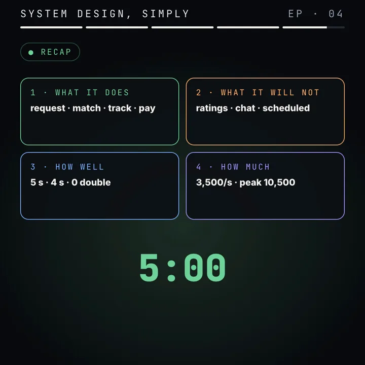
Functionally: request a ride and get a driver or a clear "none available", one driver per ride, live position, pay exactly once; ratings, chat and scheduled rides out. SLOs over 30 days: 99% of matches answered within 5 s at the gateway, 99% of map renders at most 8 s old, booking 99.9% available (43.2 minutes or 30,000 failed bookings of budget), and payments as an invariant with daily reconciliation. Estimates: one million rides a day is 11.6 a second, about 35 at a 3 times peak; with 100,000 drivers online sending every 4 s, location is 25,000 writes a second, about 720 per new ride. Bookings fit one relational database with conditional updates. The deep dive is location: latest position in memory with a TTL and a geohash or H3 index, the trail batched to durable storage, payments behind an idempotency key in a strongly consistent store.
Practice
BeginnerWhat is the error budget of a 99.95% SLO over 30 days?
0.0005 × 43,200 min = 21.6 minutes.
IntermediateGateway 99.99%, matcher 99.9%, database 99.99%, all in series. What is the end-to-end availability, and what limits it?
0.9999 × 0.999 × 0.9999 ≈ 0.9988, about 99.88%. The matcher limits it; improving the other two barely moves the result.
IntermediateWhy is the freshness SLO 8 s when phones send every 4 s?
Network jitter and the occasional lost update would break a 4 s target constantly. Allowing two intervals measures what the rider sees while tolerating one lost update.
IntermediateRides last 30 minutes instead of 20. How many rides are in progress at peak?
Little's law: 11.6 rides/s × 1,800 s ≈ 20,833 on average, × 3 ≈ 62,500 at peak.
Advanced2% of a 30-day error budget burned in one hour. What is the burn rate and how long until the budget is gone?
Burn rate 0.02 × 720 h = 14.4. At that rate the whole budget lasts 720 ÷ 14.4 = 50 hours.
AdvancedWhy can you not simply set a TTL on each driver inside a Redis geo set?
A geo index is one sorted set, and expiry applies to whole keys. Use a per-driver key with a TTL for liveness and sweep the set by last-seen time, or bucket geo keys by cell and short time window so whole buckets expire.
AdvancedA match call fans out to 20 cell shards in parallel, each slow 1% of the time. How often is the match slow, and what do you change?
1 − 0.9920 ≈ 18.2%. Search fewer shards (partition so nearby cells share a shard), require p99.9 from each shard, or send a hedged request to a replica when a shard is slow.
Cheat sheet
| Term or formula | Meaning |
|---|---|
| Functional requirement | An action and its outcome, checkable with one request |
| Non-functional requirement | A quality, checkable only statistically over many requests and time |
| SLI | good events ÷ valid events, at a stated measurement point |
| SLO | Internal target for an SLI over a window: 99% over 30 days |
| SLA | Customer contract, looser than the SLO, with a penalty |
| Error budget | (1 − SLO) × window: 99.9% over 43,200 min = 43.2 min |
| Burn rate | Share of budget used ÷ share of window elapsed; 14.4 empties 30 days in 50 h |
| Serial availability | A1 × A2 × … × An |
| Parallel availability | 1 − (1 − A)n, independent failures only |
| Fan-out tail | P(slow) = 1 − pn; 100 calls at p99 gives 63.4% |
| Little's law | L = λ × W: in progress = arrival rate × time in system |
| Node count | ceil(peak ÷ (per-node capacity × utilisation)) + 1 |
| Queueing delay (M/M/1) | wait ≈ ρ ÷ (1 − ρ) service times: 1 at 50%, 9 at 90% |
| Geohash | Interleaved lat/lon bits, 5 per character; length 6 ≈ 1.22 × 0.61 km |
| H3 | Hexagon cells, 16 resolutions; res 8 ≈ 0.737 km², ring k = 3k(k + 1) + 1 cells |
| Idempotency key | Client-made unique id; a repeat returns the stored result |
Further reading
- Google SRE book, Service Level Objectives: choosing SLIs, percentiles, SLI vs SLO vs SLA.
- Google SRE book, Embracing Risk: the cost of each nine and why error budgets exist.
- Google SRE workbook, Implementing SLOs: worked SLI specifications, measurement points and windows.
- Latency numbers every programmer should know: the orders of magnitude behind node estimates.
- AWS Well-Architected Reliability Pillar: failure domains and independent redundancy.
- H3 documentation: resolutions, cell areas, ring operations.
- Redis geospatial indexes: GEOADD, GEOSEARCH and their complexity.
This is a simplified, general explanation of common patterns using a typical ride app design, not a description of any one company's private systems. Numbers marked assumed are illustrations for practice.
Frequently asked questions
What is the difference between an SLI, an SLO and an SLA?
An SLI is a measured ratio, such as matches answered within 5 s divided by all valid match requests. An SLO is the internal target for it over a window, such as 99% over 30 days. An SLA is a contract with customers that names a looser target and a penalty.
How do you calculate an error budget?
Multiply (1 − SLO) by the window. 99.9% over a 30-day window of 43,200 minutes allows 43.2 minutes of bad time, or 0.1% of requests: 30,000 failed bookings out of 30 million.
How do you combine availability of components?
Components in series multiply: 99.99% × 99.95% × 99.99% ≈ 99.93%. Redundant copies in parallel give 1 − (1 − A)^n: two independent 99.9% copies give 99.9999%, but only if they do not fail together.
How do you estimate capacity in a system design interview?
Go from users or events per day to an average rate (divide by 86,400), multiply by a peak factor, then derive storage (rate × bytes × retention × replicas), bandwidth (rate × bytes on the wire) and nodes (peak ÷ per-node capacity × target utilisation, plus one spare).
Why is a ride app's location store different from its booking database?
Location is 25,000 small overwrites a second of data that is useless after a few seconds, so it fits an in-memory store keyed by driver with a TTL and a geospatial index. Bookings are about 35 a second and must be exact, so they go to a strongly consistent database.
What are geohash and H3?
Both split the Earth into cells with ids, so a nearby search becomes a lookup of a few cells. Geohash uses rectangles from interleaved latitude and longitude bits; H3 uses hexagons whose neighbours are all the same distance away.
Sources
- Google SRE book: Service Level Objectivessre.google
- Google SRE book: Embracing Risk (availability targets)sre.google
- Google SRE workbook: Implementing SLOssre.google
- Latency numbers every programmer should knowgist.github.com
- AWS Well-Architected Framework: Reliability Pillardocs.aws.amazon.com
- H3 documentation: hexagonal hierarchical geospatial indexh3geo.org
- Redis documentation: geospatial indexesredis.io
Linked from
- 50K fans, 5K seats. Design it.Part 1 · Performance vs scalability
- Two fans click the same seat at the same moment. Who wins?Part 2 · Race conditions and strong consistency
- Design Instagram's feed: system design in five stepsPart 3 · What system design is: the 5 steps
- Fast for you, slow for a million. Why?Part 5 · Performance vs scalability, measured
- A highway with 10 lanes can still be slowPart 6 · Latency vs throughput, measured

Written by a software engineer and system architect with 10+ years of building production web, payment, ticketing and accounting systems in Japan and Nepal. About us