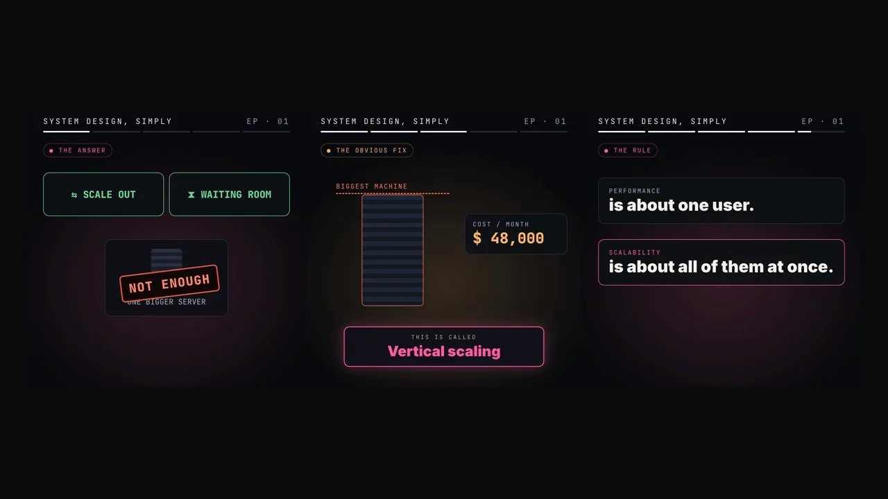
50K fans, 5K seats. Design it.
Performance vs scalability for engineers: Little's law, utilisation vs queueing delay, Amdahl and the USL, load balancing, retry storms and admission control.
 Video · 60 secondsWatch the short versionSame diagrams and numbers. Tap to play.
In this lesson you will learn
- How a ticket sale overloads one server
- Why a server slows down sharply once it is about 70% busy
- Why each extra server buys you a bit less
- How to scale out with stateless servers
Builds on Lesson 4: Latency vs throughput, measured 18 min read + 60 s video Next: CAP theorem: consistency vs availability during a partition
Drafted with AI assistance, then checked and edited by a human engineer · How we write
Short answer
Performance is the latency of one request at low load; scalability is how throughput and latency behave as load and resources grow. Queueing delay rises like ρ/(1−ρ) in the M/M/1 model, so run near 70% busy. Contention and coherency (the USL) cap what more nodes buy you. Scale out stateless servers behind a load balancer, protect the database, and admit load at the rate the slowest part can serve.
| Little's law | L = λW: items in flight = arrival rate × time in system, for any stable system |
|---|---|
| Queueing delay | M/M/1: Wq = S·ρ/(1−ρ), so 9× service time at 90% busy, 99× at 99% |
| Amdahl | Speedup = 1/((1−p) + p/N); 95% parallel caps at 20× however many cores |
| USL | X(N) = λN/(1 + σ(N−1) + κN(N−1)); peak at N* = √((1−σ)/κ) |
| Scale out needs | Stateless app tier, shared session store, idempotent requests |
| Admission control | Token bucket or waiting room sized from the slowest tier, 503 with Retry-After beyond it |
| Tail fan-out | 1% slow per backend, fan-out of 100: 1 − 0.99^100 ≈ 63% of requests are slow |
A system that answers one request in 200 ms can still fail at load. Latency depends on utilisation, and throughput is limited by contention and coordination as well as by code speed. This reference covers the queueing maths, the scaling laws and the mechanisms (load balancing, statelessness, admission control) that decide which one you have. Interview question: 50,000 users hit one endpoint within five seconds; design it so it keeps working.
Prerequisites
A request and its service time. A request is one unit of work sent to a server. Its service time is how long the server spends working on it, not counting time waiting in line before work starts. Everything below separates time in service from time in queue.
Percentiles. The p99 latency is the value 99% of requests finish within. Averages hide the slow tail, which is where load problems show up first.
Steady state. Most formulas here assume work leaves as fast as it arrives over a long window. If arrivals exceed capacity for long, queues grow until something times out or runs out of memory. Turning functional and non-functional requirements into numbers is covered in requirements, SLOs and capacity estimation for a ride app; this article assumes you already have a target load and a latency objective.
Definitions
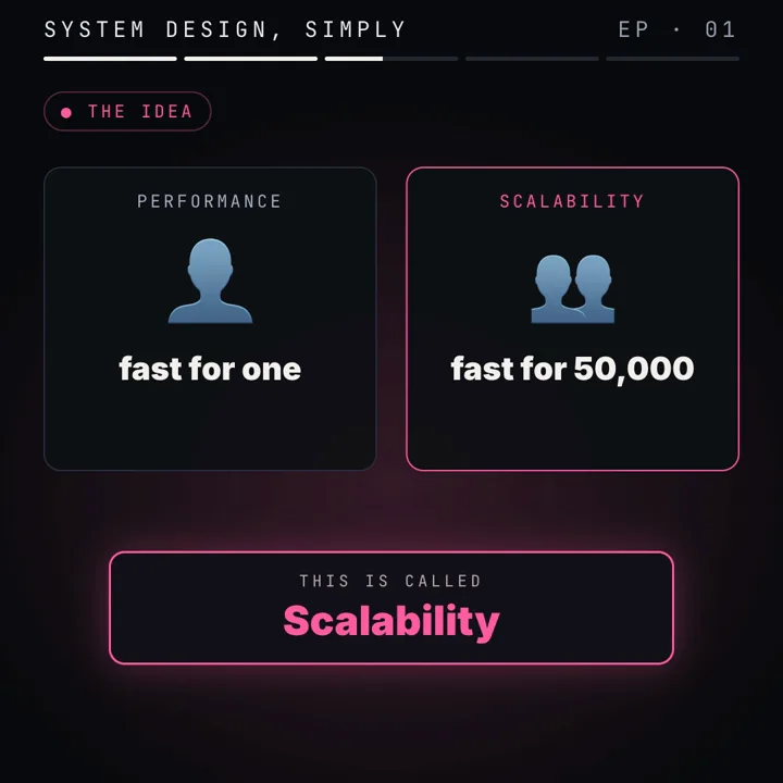
Latency: the time from sending a request to receiving the complete response, equal to queueing time plus service time (plus network time). Report it as a distribution (p50, p95, p99), not a mean.
Throughput: completed requests per unit time, X. Offered load (arrival rate, λ) is what clients send; throughput is what the system finishes. They are equal only while the system keeps up.
Utilisation: the fraction of time a resource is busy, ρ = λ × S for one server with mean service time S, or ρ = λS / c for c identical servers. A stable queue needs ρ < 1.
Performance problem: latency is too high even at low load. Test: send requests one at a time; if p95 already misses the objective, the cost is in the work itself (algorithm, query plan, a slow dependency).
Scalability problem: latency is fine alone but degrades with concurrency, or throughput stops growing as you add resources. Test: step the load (or the node count) and plot throughput and p99; a flattening throughput curve with rising p99 is the signature.
Scalability: how throughput X(N) grows as resources N grow while latency stays within objective. Linear scalability means X(N) = N × X(1); real systems fall below it.
Admission control: deciding at the entry point how much work to accept, so the system operates at a throughput it can sustain instead of collapsing under work it cannot finish.
How it works: queues, utilisation and Little's law
Every server is a queue in front of a worker pool. When requests arrive faster than workers become free, they wait. Two results explain most load behaviour.
Little's law
L = λW: the average number of items in a system equals the average arrival rate times the average time each item spends in it. It holds for any stable system regardless of arrival distribution or scheduling order. Apply it to requests in flight: a server finishing 2,000 requests a second at 0.2 s each holds 2,000 × 0.2 = 400 requests at once. If a dependency slows and W becomes 2 s at the same rate, in-flight work becomes 2,000 × 2 = 4,000. Traffic did not change, yet you need ten times the workers, connections and memory. This is how a slow database exhausts a web tier that is barely using its CPU.
The same law sizes pools. A database pool serving 3,000 queries a second at 5 ms each needs 3,000 × 0.005 = 15 connections busy on average; connections beyond that add contention without adding throughput.
Utilisation versus waiting time
The simplest queueing model, M/M/1, assumes Poisson arrivals (independent, memoryless), exponentially distributed service times, one server and first come, first served. Under those assumptions, with mean service time S and utilisation ρ:
M/M/1 model (assumptions: Poisson arrivals, exponential service, 1 server, FIFO)
  mean wait in queue      Wq = S × ρ / (1 − ρ)
  mean time in system     W  = S / (1 − ρ)
  mean queue length       Lq = ρ² / (1 − ρ)
  p99 time in system      = W × ln(100) ≈ 4.6 × W   (time in system is exponential here)
Plugging in a service time of 4 ms (assumed):
| Utilisation ρ | Wq / S = ρ/(1−ρ) | Mean W (S = 4 ms) | Lq | p99 W |
|---|---|---|---|---|
| 50% | 1.0 | 8.0 ms | 0.5 | 36.8 ms |
| 70% | 2.3 | 13.3 ms | 1.6 | 61.4 ms |
| 90% | 9.0 | 40.0 ms | 8.1 | 184 ms |
| 95% | 19.0 | 80.0 ms | 18.1 | 368 ms |
| 99% | 99.0 | 400 ms | 98.0 | 1,842 ms |
The curve is a hockey stick. From 50% to 70% the mean only goes from 2 to 3.3 service times; from 90% to 99% it goes from 10 to 100. Real servers are not M/M/1: a multi-core machine behaves more like M/M/c, which queues less at the same utilisation, and real service times are often more variable than exponential, which queues more. The shape survives both corrections: waiting time is a function of 1/(1−ρ) and explodes as ρ approaches 1.
That is the reason for running a fleet near 70% at peak. It is a rule of thumb, not a law: it keeps you on the flat part of the curve, absorbs short bursts (Poisson traffic at 70% average has many seconds above 90%), and leaves room to lose a node: if one of ten servers dies, the other nine move from 70% to about 78%, still below the knee.
Scaling laws: Amdahl and the USL
Amdahl's law
If a fraction p of the work can run in parallel and 1 − p is serial, the speedup on N processors is:
Speedup(N) = 1 / ((1 − p) + p / N)
  p = 0.95, N = 8    → 1 / (0.05 + 0.11875)   = 5.93×
  p = 0.95, N = 64   → 1 / (0.05 + 0.01484)   = 15.4×
  p = 0.95, N → ∞    → 1 / 0.05               = 20×  (hard ceiling)
In a web system the serial fraction is anything every request must pass through one at a time: a global lock, a single primary database row such as an inventory counter, a single-threaded queue consumer. Five percent serial work caps you at twenty times one node, however many you buy.
The Universal Scalability Law
Amdahl models contention (waiting for a shared resource) but assumes extra nodes never make things worse. The Universal Scalability Law (USL) adds coherency: the cost of nodes keeping each other consistent, such as cache invalidation, lock traffic, distributed coordination or replicas exchanging state. That cost grows with the number of pairs of nodes, so it is quadratic:
X(N) = λN / (1 + σ(N − 1) + κN(N − 1))
  λ  throughput of one node
  σ  contention coefficient (serialisation, 0 ≤ σ ≤ 1)
  κ  coherency coefficient (crosstalk between nodes, κ ≥ 0)
  peak at N* = √((1 − σ) / κ)
With κ = 0 this is Amdahl's law in throughput form. With κ > 0 the curve has a maximum and then falls. Example, with λ = 2,000 req/s, σ = 0.05 and κ = 0.001 (all assumed):
| Nodes N | Relative capacity | Throughput |
|---|---|---|
| 1 | 1.00 | 2,000 req/s |
| 8 | 5.69 | 11,380 req/s |
| 16 | 8.04 | 16,080 req/s |
| 31 (N* = √950 ≈ 30.8) | 9.04 | 18,076 req/s |
| 64 | 7.82 | 15,644 req/s |
Doubling from 31 to 64 nodes loses about 2,400 req/s. Fit σ and κ by measuring throughput at several node counts and regressing; the model then shows where hardware stops paying. Practically: drive κ down by removing shared mutable state between nodes (stateless app servers have κ close to zero among themselves), and drive σ down by removing hot locks and hot rows, which is the subject of race conditions, atomic updates and holds on a single seat.
Scaling up, scaling out, and what scaling out requires
Vertical scaling and its limits
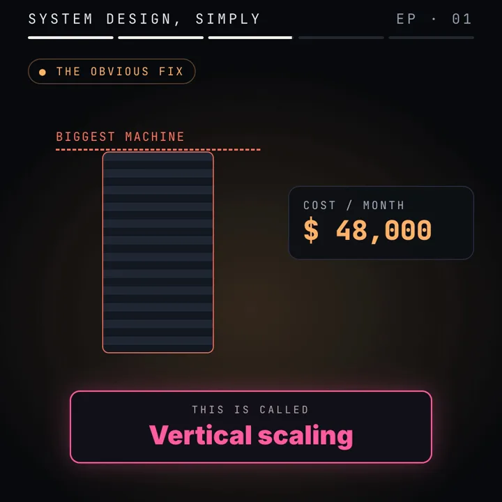
Vertical scaling (scaling up) gives one machine more cores, memory or faster storage. It needs no code change and is usually the right first step, especially for a database. Its limits:
- Cores and Amdahl. More cores help only the parallel fraction, and lock contention inside the process grows with thread count.
- Memory bandwidth and NUMA. Large servers have several sockets, each with local memory. Access to another socket's memory (non-uniform memory access, NUMA) is slower, so a process that is not NUMA-aware can get less than linear gains from the second socket. Memory bandwidth, not core count, often limits data-heavy work.
- Kernel and descriptor limits. Every socket is a file descriptor; the per-process limit (
ulimit -n) is commonly 1,024 by default. A proxy opening connections to one upstream address is bounded by the ephemeral port range (Linux default 32768 to 60999, 28,232 ports per source address and destination tuple); connections in TIME_WAIT hold ports after close. - Size and failure. There is a largest instance, and one machine means a hardware fault or a restart takes the service down.
Horizontal scaling and its prerequisites
Horizontal scaling (scaling out) adds machines and spreads requests across them. It only works if any node can serve any request, which imposes three requirements:
- A stateless app tier. No user state lives in one process's memory between requests. Sessions go into a shared store such as Redis or into a signed, expiring cookie. Sticky sessions (pinning a user to one node) are a workaround with two costs: they unbalance load, and sessions on a failed node are lost.
- Shared state with its own scaling story. Moving state out of the app tier puts it in a database, cache or queue. That tier now carries the total load of every app node, so it becomes the next bottleneck (below).
- Idempotent requests. Load balancers and clients retry. A request that timed out may or may not have run. If running it twice charges a card twice, retries are unsafe. Reads are naturally idempotent; writes need an idempotency key stored with the result so a repeat returns the first answer.
Load balancer internals
A load balancer is one address in front of many backends. Two families exist. An L4 balancer works at the transport layer: it picks a backend per TCP connection (or UDP flow) using addresses and ports, never reads HTTP, and is very cheap per packet. An L7 balancer terminates the connection, parses HTTP, and picks a backend per request, which allows routing by path or header, TLS termination, retries and per-request metrics, at more CPU per request. With long-lived connections, L4 balancing stays uneven because one connection carries many requests.
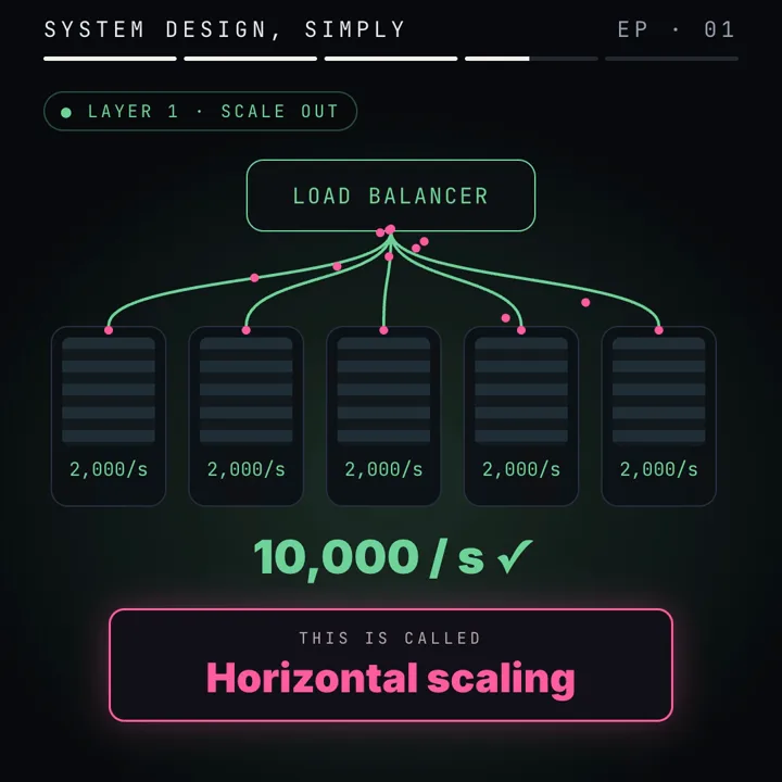
Algorithms. Round robin hands requests out in turn, optionally weighted; it is fair only when requests cost the same. Least connections sends each request to the backend with the fewest active connections, which by Little's law tracks backends that are slow right now, so it adapts to uneven request cost. Hash-based methods (client address, a header, consistent hashing) keep a key on one backend, which is useful for caches but reintroduces imbalance. "Power of two choices" (pick two at random, send to the less loaded) gets most of the benefit of least connections without global state across many balancers.
Health checks. Passive checks mark a backend down after real requests fail. In open source nginx that is max_fails failures within fail_timeout, after which the server is skipped for fail_timeout. Active checks send synthetic probes on a schedule; in nginx the health_check directive is part of the commercial subscription, while HAProxy and cloud balancers include it.
Connection draining. Removing a backend for a deploy must not cut requests in flight. The balancer stops sending new requests, lets existing ones finish up to a deadline, then removes the node. In nginx a configuration reload does this per worker: old workers finish their current requests while new workers use the new upstream list. The upstream reference also documents a drain parameter and the version that brought it to open source.
Retries at the balancer. nginx's proxy_next_upstream passes a failed request to the next server on errors and timeouts by default, but it does not resend non-idempotent methods (POST, LOCK, PATCH) once they reached a backend unless you add non_idempotent. Cap it with proxy_next_upstream_tries.
The database, retry storms and admission control
The database as the next bottleneck
Scaling the app tier multiplies load on whatever it shares. Each PostgreSQL connection is a separate backend process with its own memory (the default max_connections is 100), so a hundred app nodes each holding a pool of 20 would ask for 2,000 connections and degrade the server through context switching and lock contention long before CPU runs out. The usual moves, in order of cost:
- Connection pooling in the app and often a pooler such as PgBouncer in front, sized by Little's law (busy connections = queries/s × query time) rather than by node count.
- Caching reads that tolerate staleness (Redis, CDN, in-process) so repeated work never reaches the database.
- Read replicas for read-heavy traffic, accepting replication lag on those reads. Writes still go to one primary.
- Partitioning writes by key when one primary is not enough; the topic of later parts. How write and read paths trade cost against each other is worked through in fan-out on read versus fan-out on write for a feed.
Retry storms and metastable failure
When a server is overloaded, errors and timeouts trigger retries, and retries are new load arriving exactly when there is least capacity. If each of three layers retries three times, one user action can become 4 × 4 × 4 = 64 attempts at the bottom layer. Worse, a timed out request may still be executing, so the server spends capacity on work whose caller has already given up. The system can then stay overloaded after the original spike has passed, because the retry traffic alone exceeds capacity: a metastable failure. The Google SRE chapter on cascading failures describes this pattern in detail.
The standard mitigations: retry at one layer only; cap attempts; use capped exponential backoff with jitter, for example full jitter, sleep = random(0, min(cap, base × 2^attempt)), so clients that failed together do not retry together; use a retry budget (for example retries may be at most 10% of requests); propagate deadlines so downstream work stops when the caller has timed out.
Admission control
The more reliable fix is to accept only the work you can finish. Options, from simplest:
- Concurrency limit. Cap requests in flight per node (Little's law gives the number: target throughput × target latency). Beyond it, refuse immediately.
- Token bucket. Tokens refill at rate r up to capacity b; each request takes one. Over any interval t, at most b + r·t requests are admitted, so r sets the sustained rate and b the allowed burst. nginx's
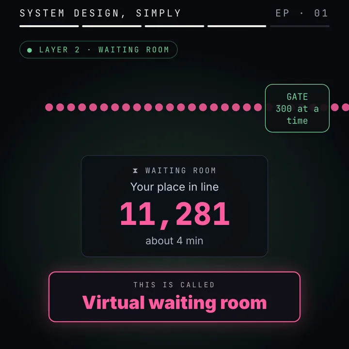
limit_reqis a leaky bucket variant of the same idea. - Waiting room. When demand exceeds capacity by an order of magnitude for minutes, refusing is a poor experience and invites refreshes. A waiting room gives each arrival a signed, ordered place and admits at a fixed rate; the protected service only ever sees the admitted rate. Polling the place must be cheap (a signature check, no database).
- Back pressure and fast refusal. When a queue is full, push back to the caller rather than buffer without bound. Refuse with
503 Service Unavailableand aRetry-Afterheader (or 429 for per-client limits), which well-behaved clients honour. A fast refusal costs microseconds; a request that queues for 30 s and then times out cost the full price and produced nothing.
Pick the admitted rate from the slowest tier, with headroom, never from the fastest.
Tail latency
A user request often fans out to many backends and waits for all of them. If each backend is slow (above its p99) 1% of the time and a request touches 100 of them, the probability that at least one is slow is 1 − 0.99100 ≈ 0.63. The backend's p99 becomes the page's typical latency. Hedged requests (send a second copy after the p95 delay, use whichever answers first), smaller fan-out and timeouts per call are the standard tools; the Tail at Scale paper in the sources is the reference. Measure p99 at the user, not only per service.
Worked example
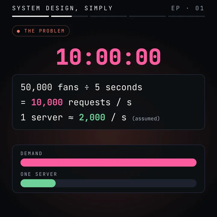
A ticket sale: 5,000 seats, 50,000 users waiting, sale opens at 10:00. All inputs below are assumed round numbers, not measurements. How to turn such numbers into estimates in general is in the step by step system design method with estimates.
Assumptions
  arrivals                 50,000 in 5 s (evenly spread)
  one app node             2,000 req/s   (8 cores × 250 req/s, 4 ms CPU each)
  target utilisation       70%
  queries per request      3
  database safe limit      3,000 queries/s
  time in shop per user    120 s,  10 requests per visit

Offered load
  50,000 / 5               = 10,000 req/s
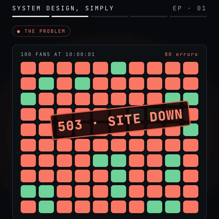
  one node                 2,000 served → 8,000 / 10,000 = 80% refused
  retry storm, second 2    10,000 new + 8,000 retries = 18,000 → 16,000 refused (89%)

App tier (scale out)
  usable per node          2,000 × 0.7 = 1,400 req/s
  nodes                    10,000 / 1,400 = 7.14 → 8, plus 1 spare = 9
  utilisation at peak      10,000 / (9 × 2,000) = 55.6%;  one node lost: 10,000 / 16,000 = 62.5%

Database without admission control
  10,000 × 3               = 30,000 queries/s  (10× the limit)

Admission control (waiting room)
  max admit rate           (3,000 × 0.7) / (10 × 3) = 2,100 / 30 = 70 users/s
  chosen rate              300 every 6 s = 50 users/s
  users in shop (Little)   L = 50 × 120 = 6,000
  shop load                6,000 × 10 / 120 = 500 req/s
  database load            500 × 3 = 1,500 queries/s  (50% of limit)
  sell-out, best case      5,000 / 50 = 100 s
  wait shown at place 11,281   11,281 / 50 = 225.6 s ≈ 3.8 min
Scaling out absorbs the arrival rate, and admission control limits the work that reaches the database, so the design needs both.
Code
1. nginx: L7 balancing, passive health checks, bounded retries, and a fast 503 with Retry-After. All directives are open source nginx; the rate limit applies per nginx instance.
# /etc/nginx/conf.d/tickets.conf
limit_req_zone $server_name zone=shop:1m rate=500r/s;   # one bucket for the whole site (constant key)

upstream ticket_app {
    least_conn;                                          # fewest active connections wins
    server 10.0.0.11:8080 max_fails=3 fail_timeout=10s;  # 3 failures in 10 s: skip for 10 s
    server 10.0.0.12:8080 max_fails=3 fail_timeout=10s;
    server 10.0.0.13:8080 max_fails=3 fail_timeout=10s;
    keepalive 64;                                        # idle upstream connections kept per worker
}

server {
    listen 80;
    server_name tickets.example.com;

    location / {
        limit_req zone=shop burst=200 nodelay;           # absorb a 200 burst, refuse beyond it
        limit_req_status 503;

        proxy_pass http://ticket_app;
        proxy_http_version 1.1;                          # required for upstream keepalive
        proxy_set_header Connection "";
        proxy_connect_timeout 1s;
        proxy_read_timeout 5s;                           # a deadline, not a hope
        proxy_next_upstream error timeout http_503;      # POST is never resent (no non_idempotent)
        proxy_next_upstream_tries 2;                     # one retry at most
    }

    error_page 503 = @busy;
    location @busy {
        add_header Retry-After 30 always;
        return 503 "Busy, retry in 30 seconds\n";
    }
}
What to observe: run a load generator such as wrk well above 500 req/s; once the burst of 200 is spent, requests get an immediate 503 with Retry-After: 30 while admitted requests keep their latency. Stop one backend: after three failures it stops receiving traffic for ten seconds.
2. Python: simulate an M/M/1 queue and check the table, then the USL curve. Standard library only.
# queue_lab.py   run: python3 queue_lab.py
import random, math

def mm1(rho, service_ms=4.0, n=200_000, seed=1):
    """Single server FIFO, Poisson arrivals, exponential service."""
    rnd = random.Random(seed)
    lam = rho / service_ms                    # arrivals per ms
    t_arrive = t_free = 0.0
    times = []
    for _ in range(n):
        t_arrive += rnd.expovariate(lam)
        start = max(t_arrive, t_free)         # wait if the server is busy
        t_free = start + rnd.expovariate(1 / service_ms)
        times.append(t_free - t_arrive)       # time in system
    times.sort()
    return sum(times) / n, times[int(0.99 * n)]

print("rho  sim_mean  model_mean  sim_p99  model_p99   (ms)")
for rho in (0.5, 0.7, 0.9, 0.95):
    mean, p99 = mm1(rho)
    w = 4.0 / (1 - rho)
    print(f"{rho:.2f} {mean:8.1f} {w:10.1f} {p99:8.1f} {w * math.log(100):10.1f}")

def usl(n, lam=2000, sigma=0.05, kappa=0.001):
    return lam * n / (1 + sigma * (n - 1) + kappa * n * (n - 1))

print("\nnodes  throughput")
for n in (1, 8, 16, 31, 64):
    print(f"{n:5d} {usl(n):11,.0f}")
print("peak at N* =", round(math.sqrt((1 - 0.05) / 0.001), 1))
What to observe: simulated means and p99 land close to the model at 50% and 70% and drift more at 95%, where the queue needs a very long run to settle; the USL output peaks near 31 nodes and falls by 64.
3. Token bucket, the core of most rate limiters:
import time

class TokenBucket:
    def __init__(self, rate, burst):
        self.rate, self.burst = rate, burst
        self.tokens, self.last = burst, time.monotonic()

    def allow(self):
        now = time.monotonic()
        self.tokens = min(self.burst, self.tokens + (now - self.last) * self.rate)
        self.last = now
        if self.tokens >= 1:
            self.tokens -= 1
            return True
        return False          # caller answers 503 or 429 with Retry-After
In production the bucket lives in a shared store (for example a Redis script) so every node draws from one limit, or each node gets rate ÷ nodes.
Failure modes and edge cases
- Thread or connection pool exhaustion with idle CPU. A dependency slows, W rises, L = λW rises past the pool size. Detect: pool wait time and in-flight count climbing while CPU is flat. Fix: timeouts per call, a bounded pool with fast refusal, circuit breaking on the slow dependency.
- Retry amplification. Detect: request rate at the lowest layer rising faster than user traffic; a high ratio of retries to first attempts. Fix: one retrying layer, retry budgets, jittered backoff, deadline propagation.
- Health check cascades. A deep health check that queries the database fails on every node during a database blip and the balancer removes all of them. Fix: shallow liveness checks; many balancers also fail open when every backend is unhealthy.
- Cold starts and autoscaling lag. New nodes take tens of seconds to minutes to boot and warm caches; a spike that builds in seconds is over before they help. Fix: scale on a schedule for known events, keep headroom, admit what the current fleet can serve.
- Uneven balance. Long-lived connections behind an L4 balancer, or hash routing on a skewed key, put most of the load on one node while the fleet average looks fine. Watch per-node utilisation, not the mean.
Trade-offs
| Option | Good for | Costs you | Use when |
|---|---|---|---|
| Vertical scaling | No code change; databases that are hard to split | Hard ceiling, NUMA and descriptor limits, single point of failure | Moderate load, or first step for a stateful tier |
| Horizontal scaling | Large, growing load; surviving node failure | Stateless design, shared state tier, idempotency, more to operate | The app tier must serve many concurrent users |
| L4 balancing | Very high packet rates, any protocol | Per-connection decisions, no HTTP awareness, uneven with long connections | Front of an L7 tier, non-HTTP traffic |
| L7 balancing | Per-request routing, retries, TLS, metrics | More CPU per request, another hop | HTTP services, most web systems |
| Read replicas and cache | Read-heavy load | Stale reads, invalidation logic | Reads dominate and tolerate lag |
| Token bucket / concurrency limit | Steady protection against bursts | Refused requests at peak | Every service, as a baseline |
| Waiting room | Demand 10× capacity for minutes | Users wait; fairness rules; one more component | Ticket drops, launches, results days |
Common mistakes
In an interview
- Clarify. Peak arrival rate and how fast it builds, read and write mix, latency objective, whether fairness matters.
- Assumptions. State node capacity, target utilisation, queries per request and database limit as labelled assumptions.
- Structure. Edge or CDN, admission control, L7 balancer, stateless app tier, session store and cache, database with pool and replicas.
- Deep dive. Offered load against capacity, node count at 70% plus a spare, Little's law for pools and in-flight work, admitted rate from the database.
- Trade-offs. Up versus out, L4 versus L7, refuse versus queue, where the USL says to stop adding nodes.
- Wrap up. Monitoring (p99, utilisation per node, retry ratio) and the next problem: concurrent writes to the same row.
"Performance is latency at low load; scalability is whether throughput grows and p99 holds as load and resources grow. 50,000 users in five seconds is 10,000 requests a second; at an assumed 2,000 per node that is 80% refused on one node. Queueing delay grows like ρ/(1−ρ), so I size at 70%: 1,400 per node, eight nodes plus a spare. Nodes are stateless behind an L7 balancer with least connections and passive health checks, sessions in Redis, writes idempotent so retries are safe. That moves the bottleneck to the database: 30,000 queries a second against a 3,000 limit. So I add admission control sized from the database, about 50 users a second through a waiting room, which by Little's law keeps it near 1,500 queries a second, and anything beyond gets a fast 503 with Retry-After. I would watch p99, per-node utilisation and the retry ratio."
Practice
BeginnerA service is slow with one user. Performance or scalability problem?
Performance. The cost is in the work itself, so optimise the code path, query or dependency before adding capacity.
IntermediateA service handles 800 req/s with mean latency 250 ms. How many requests are in flight?
Little's law: L = λW = 800 × 0.25 = 200.
IntermediateIn the M/M/1 model, how many service times does a request wait in queue at 80% utilisation?
ρ/(1−ρ) = 0.8 / 0.2 = 4 service times, so mean time in system is 5 service times.
IntermediateTen nodes run at 70%. One fails. What is the new utilisation?
Load is 10 × 0.7 = 7 node-equivalents spread over 9 nodes: 7 / 9 ≈ 77.8%.
Advanced90% of a job is parallel. What is the maximum speedup, and what do 10 cores give?
Ceiling 1 / 0.1 = 10×. With 10 cores: 1 / (0.1 + 0.09) = 5.26×.
AdvancedUSL fit gives σ = 0.02 and κ = 0.0005. Where does throughput peak?
N* = √((1 − 0.02) / 0.0005) = √1,960 ≈ 44 nodes. Beyond that, adding nodes lowers throughput.
AdvancedWhy does nginx not resend a POST to the next upstream by default?
The first backend may have executed it before failing. Resending a non-idempotent request could repeat a side effect such as a payment, so it needs the explicit non_idempotent flag, which is only safe with idempotency keys.
AdvancedEach of 50 backends is slow 1% of the time. What fraction of fan-out requests touching all 50 are slow?
1 − 0.9950 ≈ 0.395, about 39.5%.
Cheat sheet
| Term or formula | Meaning in one line |
|---|---|
| Latency | Queueing time plus service time; report p50, p95, p99 |
| Throughput X | Completed requests per second |
| Utilisation ρ = λS / c | Fraction of time busy; must stay below 1 |
| Little's law L = λW | In flight = arrival rate × time in system, any stable system |
| M/M/1 Wq = Sρ/(1−ρ) | Queue wait explodes as ρ → 1 (model assumptions apply) |
| Amdahl 1/((1−p) + p/N) | Serial fraction caps speedup at 1/(1−p) |
| USL λN/(1 + σ(N−1) + κN(N−1)) | Contention and coherency; peak at √((1−σ)/κ) |
| Vertical scaling | Bigger machine; ceiling and single point of failure |
| Horizontal scaling | More machines; needs stateless nodes and idempotency |
| L4 / L7 balancer | Per connection by address / per request by HTTP content |
| Least connections | Send to the backend with fewest requests in flight |
| Connection draining | Stop new requests, finish in-flight ones, then remove |
| Token bucket | Admits at most b + r·t requests in any interval t |
| Backoff with jitter | sleep = random(0, min(cap, base × 2^attempt)) |
| 503 + Retry-After | Fast refusal that tells clients when to come back |
| Tail fan-out | P(any slow) = 1 − (1 − p)^n |
Further reading
- NGINX load balancer guide: methods, passive health checks, session persistence.
- ngx_http_upstream_module: every
serverparameter and which are open source. - SRE book, Handling Overload: per-client limits, criticality, client-side throttling.
- SRE book, Addressing Cascading Failures: retry amplification, deadlines, load shedding.
- Timeouts, retries, and backoff with jitter: choosing timeouts and jittered backoff.
- The Tail at Scale: fan-out, tail latency and hedged requests.
This is a simplified explanation of common, general design patterns using round, assumed numbers. It is not a description of any specific company's private systems.
Frequently asked questions
What is the measurable difference between a performance problem and a scalability problem?
Measure latency at one request at a time. If it is already too slow, it is a performance problem. If it is fine alone but p99 latency or the error rate degrades as concurrent load rises, or throughput stops growing when you add resources, it is a scalability problem.
Why do teams run servers at around 70% utilisation?
Queueing delay grows like ρ/(1−ρ). In the M/M/1 model the wait is 2.3 service times at 70%, 9 at 90% and 99 at 99%. Headroom near 70% keeps latency flat, absorbs bursts and lets the fleet lose a node without saturating.
Can adding servers make a system slower?
Yes. The Universal Scalability Law adds a coherency term that grows with N(N−1), the cost of keeping nodes in agreement. Past N* = √((1−σ)/κ), each extra node lowers total throughput.
Why must retries be idempotent?
A load balancer or client cannot tell whether a timed out request was executed. If a retry can run the same purchase twice, retries are unsafe, so non-idempotent requests need an idempotency key or must not be retried automatically.
What is admission control?
Deciding at the edge how much work to accept, so the system runs at the throughput it can sustain. A token bucket, a concurrency limit or a virtual waiting room admits work; the rest is queued outside or refused fast with 503 and Retry-After.
Why look at p99 instead of the average?
Averages hide the slow requests users actually notice, and when one page fans out to many backends the slowest one sets the page time, so per-backend tails become common page-level latency.
Sources
- NGINX: Using nginx as HTTP load balancernginx.org
- NGINX: ngx_http_upstream_module referencenginx.org
- Google SRE book: Handling Overloadsre.google
- Google SRE book: Addressing Cascading Failuressre.google
- Amazon Builders' Library: Timeouts, retries, and backoff with jitteraws.amazon.com
- Google Research: The Tail at Scaleresearch.google
Linked from
- Two fans click the same seat at the same moment. Who wins?Part 2 · Race conditions and strong consistency
- Design Instagram's feed: system design in five stepsPart 3 · What system design is: the 5 steps
- 1M rides a day. What do you do in the first 5 minutes?Part 4 · Requirements in depth
- Fast for you, slow for a million. Why?Part 5 · Performance vs scalability, measured
- A highway with 10 lanes can still be slowPart 6 · Latency vs throughput, measured

Written by a software engineer and system architect with 10+ years of building production web, payment, ticketing and accounting systems in Japan and Nepal. About us