Fast for you, slow for a million. Why?
A 5 ms server against a 15 ms server: why the faster one has a 498 ms median at 100 users, explained with queueing laws, pools and a simulation.
 Video · 60 secondsWatch the short versionSame diagrams and numbers. Tap to play.
In this lesson you will learn
- The difference between performance and scalability
- Why the fastest design for one user can be the slowest for many
- How to measure both yourself with a small simulation
Builds on Lesson 2: Requirements in depth 19 min read + 60 s video Next: Latency vs throughput, measured
Drafted with AI assistance, then checked and edited by a human engineer · How we write
Short answer
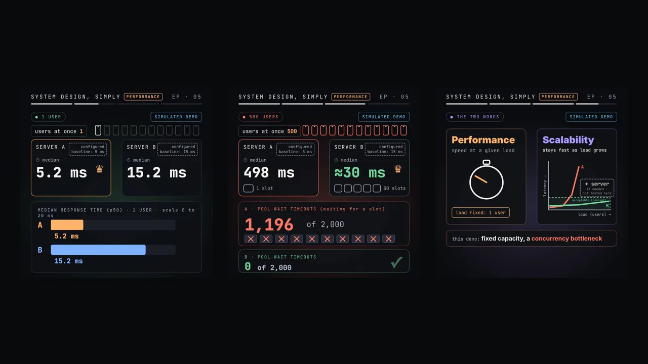
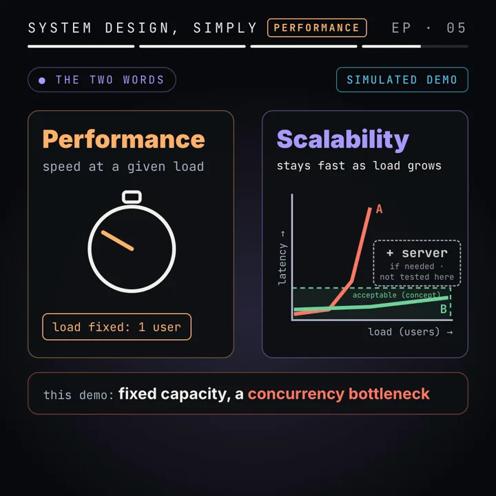
Performance is how fast one request is at a given load; scalability is whether it stays acceptably fast as load grows. In our simulation, A (5 ms of work, 1 connection) beat B (15 ms, pool of 50) with one user, 5.2 vs 15.2 ms median. At 100 users A's median was 498.1 ms and B's 29.8 ms, because A tops out at 1 ÷ 5 ms = 200 req/s and B at 50 ÷ 15 ms, about 3,333.
| Throughput ceiling | X_max = connections ÷ work per request: A 1 ÷ 0.005 s = 200 req/s, B 50 ÷ 0.015 s ≈ 3,333 req/s |
|---|---|
| Response time law | Closed loop, no think time: R = N ÷ X, so 100 users ÷ 200.4 req/s ≈ 0.5 s for A |
| 1 user (simulated) | Median 5.2 ms for A vs 15.2 ms for B: A has better performance |
| 100 users (simulated) | Median 498.1 vs 29.8 ms, p99 509.1 vs 33.7 ms: B scales, A queues |
| Throughput (simulated) | A peaked at 200.6 req/s, B at 3,299.1 req/s |
| 500 users (simulated) | A: 1,196 of 2,000 requests hit the 1 s pool-wait timeout; B: 0 |
| Crossover | A was already slower at 10 users, the first tested level above 1 |
A request that takes 5 ms on an idle server can take half a second when 100 people send it at once, while a slower 15 ms design stays near 30 ms. The difference comes from how many requests each design can work on at the same time, and this article measures it in a small simulation, derives every number from two formulas, and shows how to find the same limit in your own system.
Prerequisites
Work time and waiting time. The time you see for a request is the time it spends being worked on plus the time it spends waiting for something to become free. On an idle server waiting time is zero, so a single-user test measures only work. Every number in this article is about separating the two.
Percentiles. The median (p50) is the latency half of the requests beat. The p99 is the latency 99% of requests beat, so it describes the slow tail that some users always see. A mean mixes both and hides the tail.
Little's law. In any stable system, the average number of items inside equals their arrival rate times the average time each one spends inside: L = λ × W. Part 1 of this series uses it to size servers and explains the queueing curve behind it in performance vs scalability for a ticket rush. Here we use the same law in reverse, to predict latency from a user count.
Definitions
Performance: how quickly a system does its work at a given load, usually reported as latency percentiles and throughput measured at that load. "Fast with one user" is a performance statement.
Scalability: the ability of a system to keep performance acceptable as load grows, adding resources if needed. This follows the framing in Microsoft's engineering playbook (see sources). A scalability statement always names a load range.
Throughput: completed requests per second. In this article, only successful requests count; requests that time out are errors.
Bottleneck: the resource with the highest demand per request relative to its parallelism. It sets the throughput ceiling for the whole path, however fast everything else is.
Connection pool: a fixed set of open database connections that requests borrow and return. A request that finds every connection busy waits in the pool's line until one is released or until its acquire timeout fires.
Saturation point (N*): the number of concurrent users at which the bottleneck becomes busy all the time. Below it, extra users add throughput; above it, extra users add only waiting time.
Closed-loop load: a fixed number of users, each sending a new request only after its previous one returns. Open-loop load: requests arrive at a set rate whatever the server is doing, the way real visitors arrive.
How it works: the ceiling and the line
Take two versions of the same endpoint. Version A does about 5 ms of work, but every request needs the one database connection the process holds. Version B does about 15 ms of work (perhaps an extra lookup, perhaps a slower query plan), and it borrows from a pool of 50 connections. Everything else is equal.
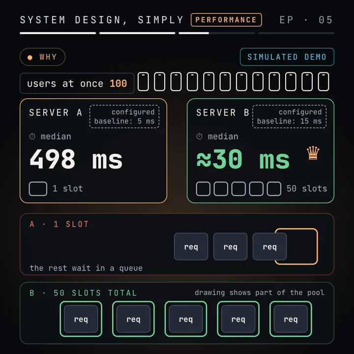
Two results from operational analysis, the branch of performance modelling that works from measured averages instead of probability distributions, are enough to predict what happens.
The throughput ceiling
A resource with c parallel slots, each held for S seconds per request, can finish at most c ÷ S requests a second. This is the utilisation law turned around: utilisation U = X × S ÷ c can never exceed 1.
X_max = c / S
  A:  1 / 0.005 s  = 200 req/s
  B: 50 / 0.015 s  ≈ 3,333 req/s     (about 16.7 times A)
B does three times more work per request and still has a ceiling about 16.7 times higher, because it can do 50 pieces of work at once against A's one. Fifty times the slots divided by three times the work gives the ratio, 50 ÷ 3.
The response time law
In a closed loop with N users and think time Z (the pause between a response and the next request), Little's law applied to the whole loop gives N = X × (R + Z). Our users send again immediately, so Z = 0 and:
R = N / XBelow saturation, X grows with N and R stays at the bare work time. Above saturation, X is pinned at X_max, so R grows in a straight line with N. Each extra user adds S ÷ c of waiting: 5 ms per user for A, 0.3 ms per user for B.
R(N) ≈ max(S, N × S / c)          (plus a small unshared overhead)
N*   ≈ c                          (with zero think time)
  A: N* ≈ 1    → saturated by a single user
  B: N* ≈ 50   → flat latency up to about 50 users
So A is already at its ceiling with one user, because that user keeps the single connection busy almost all the time, and every additional user waits. B has headroom for about 50 users before anyone waits at all.
Where the lines cross. A's latency is about 5 × N ms and B's stays at 15 ms until N reaches 50, so A becomes slower once 5N passes 15. The formula puts the crossover at 4 users. That is a prediction; the simulation tested 1, 10, 100 and 500 users and found A already slower at 10.
What the simulation measured
To check the formulas we wrote a discrete-event simulation: a program that keeps a virtual clock and a list of timed events (request arrives, connection freed, timeout fires) and jumps from one event to the next. There is no real database, HTTP server or network, and the laptop's speed does not affect the numbers. It runs in Node.js with a fixed random seed (42), 2,000 requests per version per user level, ±20% jitter on the work time, 0.2 ms of unshared handling overhead and a 1,000 ms limit on waiting for a connection. It shows the shape of queueing behaviour, not the capacity of any real system.
| Users | A p50 | A p99 | A req/s | B p50 | B p99 | B req/s |
|---|---|---|---|---|---|---|
| 1 | 5.2 ms | 6.2 ms | 192.2 | 15.2 ms | 18.1 ms | 65.7 |
| 10 | 50.2 ms | 54.2 ms | 199.4 | 15.2 ms | 18.1 ms | 654.3 |
| 100 | 498.1 ms | 509.1 ms | 200.4 | 29.8 ms | 33.7 ms | 3,299.1 |
| 500 | 999.8 ms | 1,004.9 ms | 200.6 | 149 ms | 154.3 ms | 3,295.4 |
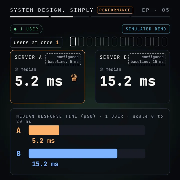
One user. A's median is 5.2 ms (5 ms of work plus 0.2 ms of overhead) and B's is 15.2 ms. If you only ever test with one user, A looks three times better. Its throughput of 192.2 req/s is already 96% of its 200 req/s ceiling: 192.2 × 0.005 s ≈ 0.96 connections busy on average.
Ten users. A's throughput rises only to 199.4 req/s, so the response time law gives 10 ÷ 199.4 ≈ 50.2 ms, exactly the measured median. The longest line for A's connection was 9 requests: everyone except the one being served. B has 10 users and 50 connections, nobody waits, its latency is unchanged at 15.2 ms and its throughput rises tenfold to 654.3 req/s.
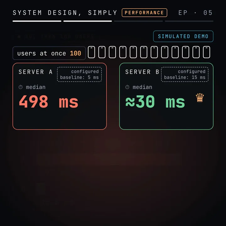
A hundred users. A is pinned at 200.4 req/s, so R = 100 ÷ 200.4 ≈ 0.499 s; measured median 498.1 ms, p99 509.1 ms. Almost all of that is waiting: 5 ms of work behind about 99 other requests. B has passed its saturation point of about 50, so it queues too (the longest line was 50 requests), and R = 100 ÷ 3,299.1 ≈ 30.3 ms against a measured median of 29.8 ms. B doubled from its idle latency; A grew almost a hundredfold.
The tail stays close to the median. At 100 users A's p99 is only 2% above its p50. When latency is mostly a long line of identical waits, every request waits about as long as every other. A wide gap between p50 and p99 usually means something else, such as a few slow queries, garbage collection pauses or a cold cache. A narrow gap at a high value suggests a single saturated resource.
The formula's predictions (5.2, 50.2, 500.2 ms for A; 15.2, 15.2, 30.2, 150.2 ms for B) are within about 1% of the measured medians. When a load test disagrees with them by much more than that, the model is missing a resource, and the next job is to find it.
What happens past the timeout
At 500 users A's predicted wait is 500 × 5 ms = 2.5 s, longer than the 1 s the pool will let a request wait. So most requests fail.
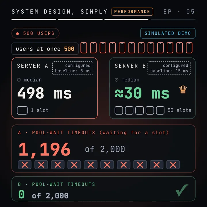
- Errors: 1,196 of A's 2,000 requests hit the pool-wait timeout, 59.8%. B had 0.
- Throughput did not fall: A still completed 200.6 successful requests a second, its ceiling. The connection never stopped working; the extra demand turned into errors instead of more output.
- Survivors are slow too: the successful requests had a median of 999.8 ms and a p99 of 1,004.9 ms. They are the ones that got a connection just before their deadline, so the timeout value itself became the latency.
- The line never shrinks: the longest line was 499 requests, every user but one. In a closed loop a timed-out user immediately sends a new request, which behaves exactly like an automatic retry.
B at 500 users is well past its own saturation point. Its median rose to 149 ms (R = 500 ÷ 3,295.4 ≈ 152 ms), the longest line was 450, and every request still finished inside the timeout. B is not limitless: by R = N × 0.3 ms its waits would cross 1 s somewhere past 3,300 users, so B also scales only over a range of load.
Two production lessons follow. A timeout protects the caller's time but does not create capacity, so it moves the failure from "slow" to "error" at the same throughput. And work that the client has abandoned should be dropped before it starts, which is why the pool checks the deadline while the request is still in line rather than after it runs. The Google SRE chapter on handling overload in the sources covers the server side of this: reject early and cheaply, and keep clients from retrying in lockstep. Retry storms, backoff with jitter and admission control are worked through in the ticket rush article on overload.
Where one slot hides in real software
Few production services literally hold one database connection. The single slot in version A stands for any resource that every request must hold, one at a time:
- A pool configured too small. HikariCP, the common Java pool, defaults
maximumPoolSizeto 10 andconnectionTimeoutto 30,000 ms. node-postgres defaults its pool to 10 connections. A service that does more than about 10 concurrent queries per instance waits in the pool, however fast the database is. - A lock around shared state. A mutex around an in-memory cache, a counter row that every write updates, or a file appended by every request. Holding the same row lock in a database is the problem covered in how an atomic update stops two fans buying one seat: correctness forces one-at-a-time, so keep the locked section as short as possible.
- A single-threaded worker. One event-loop thread doing CPU-heavy JSON parsing or image work, or one queue consumer. Its ceiling is 1 ÷ (CPU time per item).
- A downstream limit. A partner API that allows a fixed number of concurrent calls, or a per-tenant rate limit. You cannot see it in your own CPU graphs.
Why the pool of 50 is not free
In the simulation, B's 50 connections are 50 independent slots. A real database has a fixed amount of CPU and disk, so the pool's ceiling is c ÷ S only while S stays at 15 ms as c grows. PostgreSQL runs a separate backend process per connection and ships with max_connections set to 100 by default. Raising the pool past what the server can actually run in parallel makes S longer (context switching, lock contention, cache misses), and the ceiling c ÷ S stops rising or falls. The HikariCP wiki on pool sizing argues for small pools for this reason and starts from a rule of thumb near (cores × 2) + effective spindle count, to be checked by load tests.
Little's law gives the right starting size. Busy connections on average = queries per second × time per query. A service that must do 3,000 queries a second at 15 ms each (assumed figures) keeps 3,000 × 0.015 = 45 connections busy on average, so a pool of 50 runs at about 90%, and a burst will queue. Many instances each holding a pool multiply the total: 20 instances (assumed) × 50 = 1,000 connections against a server whose default limit is 100. A pooler such as PgBouncer in transaction mode lets many client connections share a smaller set of server connections (its default_pool_size is 20 per user and database pair), which keeps the database side bounded while instances scale out.
Finding the bottleneck in a live system
- Look for saturation, not speed. For each resource on the request path, record utilisation (busy time ÷ wall time) and queue length: pool active and pending counts, lock wait time, thread pool queue, CPU run queue.
- Find the largest demand. For each resource compute S ÷ c, the time per request divided by parallel slots. The largest value is the bottleneck, and c ÷ S is the service's ceiling.
- Confirm with a step test. Raise concurrency in steps. If throughput flattens near the predicted ceiling while latency grows by S ÷ c per added user, you found it.
Pool metrics make this easy: HikariCP exposes active, idle and pending connection counts, and PgBouncer's SHOW POOLS lists clients waiting for a server connection. A steady non-zero pending count with a flat throughput graph is the signature of version A.
Closed-loop and open-loop load tests
The simulation is closed loop: 100 users means at most 100 requests in the system, and a slow server automatically receives fewer requests per second. That is why A's latency grew in a straight line and stopped there. Real traffic is often closer to open loop: visitors arrive whether or not the server is keeping up.
| Property | Closed loop | Open loop |
|---|---|---|
| Load set by | Number of users N | Arrival rate λ |
| Above the ceiling | Latency = N ÷ X_max, bounded | Line grows by λ − X_max per second, unbounded |
| Fits | Batch workers, connection-limited clients, a fixed set of services | Public web traffic, mobile apps, webhooks |
| Risk when testing | Hides latency, because a slow response delays the next request (coordinated omission) | Needs a generator that sends on schedule even while responses are slow |
Run version A open loop at 300 requests a second (an assumed rate) and the line grows by about 100 requests every second until timeouts or memory end it. The same server that showed a tidy 498.1 ms median in a closed test would show nothing but timeouts. Gil Tene named the measurement error "coordinated omission": a load generator that waits for each response skips exactly the requests that would have seen the worst latency. When you load test a public endpoint, use a tool mode that keeps a constant arrival rate, and report the rate you offered next to the rate you achieved.
Worked example
The video's scenario: the same endpoint, two designs, and a crowd that grows from one user to 500. All inputs are configuration of the simulation; all results come from its output.
CONFIG     A: 5 ms work, 1 connection     B: 15 ms work, 50 connections
           jitter ±20%, overhead 0.2 ms, wait limit 1,000 ms, 2,000 requests per level

CEILING    A: 1 / 0.005 s  = 200 req/s     measured max 200.6 req/s
           B: 50 / 0.015 s ≈ 3,333 req/s   measured max 3,299.1 req/s

1 USER     A: 5 + 0.2      = 5.2 ms        measured p50 5.2 ms
           B: 15 + 0.2     = 15.2 ms       measured p50 15.2 ms

100 USERS  A: 100 / 200.4  ≈ 499 ms        measured p50 498.1 ms, p99 509.1 ms
           B: 100 / 3,299.1 ≈ 30.3 ms      measured p50 29.8 ms, p99 33.7 ms

500 USERS  A: 500 × 5 ms   = 2,500 ms > 1,000 ms limit
                                           measured 1,196 of 2,000 timed out
           B: 500 / 3,295.4 ≈ 152 ms       measured p50 149 ms, 0 timed out

CROSSOVER  5 × N > 15  →  N ≥ 4 predicted; first tested level where A is slower: 10
Pick between the designs by comparing each ceiling with expected traffic; one-user latency matters only below the ceiling. If the endpoint will see a few requests a second, A is the better design: lower latency and fewer connections. If it will see hundreds a second, A cannot serve them at any latency, and B's extra 10 ms per request buys about 16 times more headroom. Turning expected traffic into a requests-per-second target is the subject of requirements, SLOs and capacity estimation.
Code
The simulation behind every measured number in this article, trimmed for reading. It is the same model as our lab script, with the same seed and event ordering, and prints the same table. Save it as pool_lab.mjs and run node pool_lab.mjs (Node.js 18 or newer, no packages, no network).
// pool_lab.mjs: two versions of one endpoint, simulated on a virtual clock.
// A: about 5 ms of work, 1 connection.  B: about 15 ms of work, pool of 50.
// Closed loop: each user sends the next request when the last one returns.
// Node.js 18+, no packages, no network. Same seed, same numbers, any machine.
const SEED = 42, REQUESTS = 2000, TIMEOUT_MS = 1000, OVERHEAD_MS = 0.2, JITTER = 0.2;
const VERSIONS = { A: { serviceMs: 5, pool: 1 }, B: { serviceMs: 15, pool: 50 } };
const USERS = [1, 10, 100, 500];

function mulberry32(seed) {               // small seeded random number generator
  let a = seed >>> 0;
  return () => {
    a = (a + 0x6d2b79f5) >>> 0;
    let t = a;
    t = Math.imul(t ^ (t >>> 15), t | 1);
    t ^= t + Math.imul(t ^ (t >>> 7), t | 61);
    return ((t ^ (t >>> 14)) >>> 0) / 4294967296;
  };
}

function simulate({ serviceMs, pool }, users, seed) {
  const rand = mulberry32(seed);
  const events = [];                       // kept sorted by (time, sequence)
  let now = 0, seq = 0;
  const at = (t, fn) => {
    const e = { t, s: seq++, fn };
    let lo = 0, hi = events.length;
    while (lo < hi) {
      const m = (lo + hi) >> 1;
      if (events[m].t < t || (events[m].t === t && events[m].s < e.s)) lo = m + 1; else hi = m;
    }
    events.splice(lo, 0, e);
  };

  let free = pool, issued = 0, waitingNow = 0, maxQueue = 0, last = 0;
  const line = [];                         // FIFO of requests waiting for a connection
  let head = 0;
  const done = [];                         // { ms, ok }

  const send = () => {
    if (issued++ >= REQUESTS) return;
    const req = { start: now, waiting: false };
    at(now + OVERHEAD_MS, () => acquire(req));   // parsing and routing, not shared
  };
  const acquire = (req) => {
    if (free > 0) { free--; serve(req); return; }
    req.waiting = true; line.push(req); waitingNow++;
    maxQueue = Math.max(maxQueue, waitingNow);
    at(now + TIMEOUT_MS, () => {           // still in line after 1 s: request fails
      if (req.waiting) { req.waiting = false; waitingNow--; finish(req, false); }
    });
  };
  const serve = (req) => {
    const ms = serviceMs * (1 - JITTER + 2 * JITTER * rand());   // +/-20%
    at(now + ms, () => { release(); finish(req, true); });
  };
  const release = () => {                  // hand the connection to the next in line
    while (head < line.length) {
      const next = line[head++];
      if (next.waiting) { next.waiting = false; waitingNow--; serve(next); return; }
    }
    free++;
  };
  const finish = (req, ok) => { done.push({ ms: now - req.start, ok }); last = now; send(); };

  for (let i = 0; i < users; i++) send();
  while (events.length) { const e = events.shift(); now = e.t; e.fn(); }

  const ok = done.filter((r) => r.ok).map((r) => r.ms).sort((a, b) => a - b);
  const pct = (p) => ok[Math.min(ok.length - 1, Math.ceil((p / 100) * ok.length) - 1)];
  const r1 = (x) => Math.round(x * 10) / 10;
  return { users, p50: r1(pct(50)), p99: r1(pct(99)), rps: r1(ok.length / (last / 1000)),
           errors: done.length - ok.length, maxQueue };
}

for (const [name, v] of Object.entries(VERSIONS)) {
  console.log(`${name}: ${v.serviceMs} ms work, pool of ${v.pool}`);
  console.log('  users    p50 ms    p99 ms     req/s   timeouts  max queue');
  USERS.forEach((u, i) => {
    const r = simulate(v, u, SEED + i);
    console.log(`  ${String(u).padStart(5)} ${String(r.p50).padStart(9)} ${String(r.p99).padStart(9)} ` +
      `${String(r.rps).padStart(9)} ${String(r.errors).padStart(10)} ${String(r.maxQueue).padStart(10)}`);
  });
}
Real output:
A: 5 ms work, pool of 1
  users    p50 ms    p99 ms     req/s   timeouts  max queue
      1       5.2       6.2     192.2          0          0
     10      50.2      54.2     199.4          0          9
    100     498.1     509.1     200.4          0         99
    500     999.8    1004.9     200.6       1196        499
B: 15 ms work, pool of 50
  users    p50 ms    p99 ms     req/s   timeouts  max queue
      1      15.2      18.1      65.7          0          0
     10      15.2      18.1     654.3          0          0
    100      29.8      33.7    3299.1          0         50
    500       149     154.3    3295.4          0        450
The prediction side, in plain Python 3, so you can compare the formula with the measurement before running any load test:
# predict.py: what the operational laws predict before you run anything.
# Closed loop with zero think time: every user always has one request in the system.
OVERHEAD_MS = 0.2                      # parse and route, done in parallel, never queued
VERSIONS = {"A": (5, 1), "B": (15, 50)}  # (work per request in ms, connections)

def ceiling_rps(service_ms, pool):
    return pool / (service_ms / 1000)  # X_max = c / S

def response_ms(users, service_ms, pool):
    # below saturation you wait only for your own work; above it, R = N / X_max
    return OVERHEAD_MS + max(service_ms, users * service_ms / pool)

for name, (s, c) in VERSIONS.items():
    print(f"{name}: ceiling {ceiling_rps(s, c):,.1f} req/s, knee at N* = {c}")
    for n in (1, 10, 100, 500):
        print(f"   {n:>3} users  predicted {response_ms(n, s, c):7.1f} ms")

first = next(n for n in range(1, 101) if response_ms(n, *VERSIONS["A"]) > response_ms(n, *VERSIONS["B"]))
print(f"A first slower at {first} users (prediction)")
A: ceiling 200.0 req/s, knee at N* = 1
1 users predicted 5.2 ms
10 users predicted 50.2 ms
100 users predicted 500.2 ms
500 users predicted 2500.2 ms
B: ceiling 3,333.3 req/s, knee at N* = 50
1 users predicted 15.2 ms
10 users predicted 15.2 ms
100 users predicted 30.2 ms
500 users predicted 150.2 ms
A first slower at 4 users (prediction)What to observe when you change the simulation:
- Set A's
poolto 3. Its ceiling becomes 3 ÷ 0.005 s = 600 req/s, and its latency at 100 users drops to about a third. More slots helped more than faster work. - Set B's
serviceMsto 10. Its one-user latency drops by a third, and its ceiling rises to 5,000 req/s. Performance work raises the ceiling too, as long as the slots stay. - Set
TIMEOUT_MSto 5000 and rerun 500 users. A's errors vanish, its median moves toward 2.5 s, and its throughput stays at its ceiling. The timeout decides whether overload shows up as errors or as latency; it does not change how much work gets done. - The prediction misses A at 500 users (2,500 ms predicted) because the 1 s limit removes requests from the line. Any model that ignores timeouts overestimates latency and underestimates errors past the ceiling.
Failure modes and edge cases
Benchmarks run with one user. A comparison at concurrency 1 measures performance only and picks version A every time. Detect it by asking for the concurrency level next to every latency figure. Fix it with a step test up to and past the expected peak.
Pool exhaustion that looks like a slow database. Application traces show 500 ms "database time" while the database reports 5 ms queries. The difference is time spent waiting for a connection inside the app. Detect with pool pending counts and acquire-time metrics, recorded separately from query time.
Scaling out multiplies connections. Adding instances to fix pool waits moves the line into the database: each instance brings a full pool, and the server's connection limit or its CPU becomes the new single slot. Detect with database connection counts and active sessions against cores. Fix with a shared pooler and smaller per-instance pools sized by Little's law.
Lock convoys. A lock held while doing slow work (a network call inside a transaction, logging under a mutex) turns S for the lock into the slow work's time. Detect with lock wait metrics or a profiler; fix by moving slow work outside the critical section.
Timeouts that do not cancel work. If the client gives up after 1 s but the server keeps running the request, the server spends its ceiling on answers nobody reads. Pass deadlines down the call chain and check them before expensive steps, the way the simulated pool drops a request whose wait has expired.
Trade-offs
| Option | Good for | Costs you | Use when |
|---|---|---|---|
| Fewer slots, faster work (A) | Lowest latency at low load, few connections, simple | Ceiling of c ÷ S; collapses into queueing above it | Traffic stays well below the ceiling, or the resource must be serial for correctness |
| More slots, slower work (B) | Throughput ceiling far above expected load | Higher idle latency; more connections and memory on the shared resource | Many concurrent users and a backend that can really run that many at once |
| Bigger connection pool | Removes waiting inside the app | Can overload the database; multiplied by instance count | Pool pending is high and database CPU and I/O have headroom |
| Shared pooler (PgBouncer, transaction mode) | Many clients on a bounded set of server connections | Session features (prepared statements, session settings) need care; one more hop | Many app instances in front of one PostgreSQL primary |
| Short acquire timeout | Fast failure, caller can fall back or retry elsewhere | More visible errors at the same throughput | Callers have a fallback, or a long wait is worse than an error |
| Admission limit at the edge | Bounded line, predictable latency for admitted work | Some users are turned away | Open-loop traffic can exceed the ceiling |
Common mistakes
Explaining it in 60 seconds
Whether you are explaining a slow release to your team or reviewing your friend's design, the same six steps keep the explanation short. (The structure also works as an answer in a system design interview.)
- Clarify: which endpoint, what load, which percentile matters.
- Assumptions: the work time per request and the number of slots it holds.
- Structure: ceiling c ÷ S, then R = N ÷ X above it.
- Deep dive: which resource is the single slot, and how you would confirm it with pool or lock metrics.
- Trade-offs: more slots against more load on the shared database, timeouts against errors.
- Wrap up: the change you would make and the step test that proves it.
Performance is how fast a request is at a given load; scalability is whether it stays acceptably fast as load grows. Version A does 5 ms of work but shares one connection, so it can finish at most 1 ÷ 5 ms = 200 requests a second, and it is saturated by a single user. Version B does 15 ms of work over a pool of 50, a ceiling of about 3,333 a second. In our simulation A won with one user, 5.2 ms against 15.2 ms median, but at 100 users its median was 498.1 ms against B's 29.8 ms, because by R = N ÷ X each of A's users waits behind about 99 others. At 500 users, 1,196 of A's 2,000 requests timed out waiting for the connection and B had none. So I look for the resource every request must hold, compute its ceiling, and compare that with peak traffic before I look at single-request speed.
Practice
BeginnerA request holds one of 8 worker threads for 20 ms. What is the throughput ceiling?
8 ÷ 0.020 s = 400 requests a second.
IntermediateVersion A runs at 200.4 req/s with 100 closed-loop users and no think time. What median latency do you expect, and why?
R = N ÷ X = 100 ÷ 200.4 ≈ 0.499 s. Every user always has one request in the system, so the line holds about 99 requests ahead of each new one. The simulation measured 498.1 ms.
IntermediateAt one user, A's throughput was 192.2 req/s. How busy was its single connection?
U = X × S = 192.2 × 0.005 s ≈ 0.96, about 96% busy. One user already saturates it, which is why a second user has to wait.
IntermediateWhy did A's throughput stay near 200 req/s at 500 users even though most requests failed?
The connection never went idle; it kept finishing 5 ms requests. The extra demand could only wait, and waits longer than 1 s became timeouts. Errors replaced latency at the same throughput.
AdvancedWith zero think time, at roughly how many users does each version saturate, and what changes if users pause 1 s between requests?
N* ≈ c with Z = 0: about 1 for A and about 50 for B. With think time, N* ≈ c × (S + Z) ÷ S, so A saturates near 1 × 1.005 ÷ 0.005 = 201 users and B near 50 × 1.015 ÷ 0.015 ≈ 3,383 users. Think time lets many more users share the same ceiling.
AdvancedTen app instances each have a pool of 50 in front of one PostgreSQL server with the default connection limit. What goes wrong, and what do you change?
They ask for 500 connections against a default max_connections of 100, so most instances fail to connect at startup or under load. Put a pooler such as PgBouncer in transaction mode in front, shrink per-instance pools, and size the server side from total queries per second × query time.
AdvancedYour closed-loop test of A at 100 users shows a stable 498 ms median. Production gets 300 requests a second arriving independently. What happens?
Arrivals exceed the 200 req/s ceiling by 100 a second, so the line grows by about 100 requests every second without bound until timeouts or memory end it. The closed-loop test hid this because slow responses slowed its own sending.
Cheat sheet
| Term or formula | Meaning |
|---|---|
| Performance | How fast the work is at a given load: latency and throughput at that load |
| Scalability | Keeping performance acceptable as load grows, adding resources if needed |
| X_max = c ÷ S | Throughput ceiling of a resource with c slots held S seconds each |
| U = X × S ÷ c | Utilisation law; a resource is saturated as U approaches 1 |
| L = λ × W | Little's law: items inside = arrival rate × time inside |
| R = N ÷ X − Z | Response time law for a closed loop with N users and think time Z |
| N* ≈ c × (S + Z) ÷ S | Saturation point; with Z = 0 it is about c |
| Bottleneck | Resource with the largest S ÷ c; it sets the ceiling of the path |
| Pool sizing | Busy connections = queries/s × time per query, plus headroom |
| Acquire timeout | Longest wait for a pooled connection; past the ceiling it turns waits into errors |
| Closed loop | Fixed users, next request after the last reply; latency bounded |
| Open loop | Fixed arrival rate; above the ceiling the line grows without bound |
| Coordinated omission | A load tool that waits for replies skips the requests that would be slowest |
Further reading
- Microsoft Code-With Engineering Playbook, Performance: the definitions of performance and scalability used here, and how to plan performance testing.
- Little (1961), Operations Research: the original proof that L = λW holds for any stable queue.
- Quantitative System Performance (Lazowska et al.): the operational laws (utilisation, response time, bottleneck bounds) behind every formula in this article, free online.
- PostgreSQL connection settings:
max_connectionsand the per-connection resources behind it. - PgBouncer configuration: pool modes and
default_pool_sizefor sharing server connections. - HikariCP, About Pool Sizing: why smaller pools often give more throughput, with a starting formula.
- Google SRE book, Handling Overload: rejecting work early and keeping clients from making overload worse.
Next in the series, part 6: why a 10 lane highway can still be slow, or the difference between latency and throughput.
This is a simplified, general explanation of common patterns, not a description of any company's private systems. All measured numbers come from our discrete-event simulation on a virtual clock (Node.js v22.13.1, seed 42, 2,000 requests per level). It models queueing only, with no real database, HTTP server or network, and does not represent the capacity of any production system.
Frequently asked questions
What is the difference between performance and scalability?
Performance is how quickly a system does its work at a given load, for example the median latency of one request with one user. Scalability is its ability to keep performance acceptable as load grows, adding resources if needed. A system can be fast for one user and still scale badly.
Why can a faster server be slower under load?
Because latency under load is mostly waiting, not working. If every request needs one shared resource, such as a single database connection, requests line up behind it. With 5 ms of work and one connection the ceiling is 200 requests a second, so 100 users each wait for about 99 others: roughly 500 ms.
How do I calculate the maximum throughput of a connection pool?
Divide the number of connections by the time each request holds one. 50 connections held for 15 ms each give 50 ÷ 0.015 s ≈ 3,333 requests a second. One connection held for 5 ms gives 200. Past that rate the extra requests wait in line.
Is a bigger connection pool always better?
No. A pool only helps if the thing behind it can do that much work at once. A PostgreSQL server runs one process per connection, so thousands of connections add memory and context switching without more throughput. Size the pool from measured query time and the database's real parallelism.
Were these numbers measured on real servers?
No. They come from a discrete-event simulation on a virtual clock (Node.js, seed 42, 2,000 requests per level), with no real database, HTTP server or network. It shows the shape of queueing behaviour, not the capacity of any production system.
What is a closed-loop load test?
A test where a fixed number of simulated users each send their next request only after the previous one returns. It caps the load at the number of users, so a slow server automatically receives fewer requests. Real traffic often keeps arriving regardless, which an open-loop test models.
Sources
- Microsoft Code-With Engineering Playbook: Performancemicrosoft.github.io
- Little, J. D. C. (1961): A Proof for the Queuing Formula L = λW, Operations Researchpubsonline.informs.org
- Lazowska et al.: Quantitative System Performance (free online book)homes.cs.washington.edu
- PostgreSQL documentation: Connections and Authentication settingspostgresql.org
- PgBouncer documentation: configurationpgbouncer.org
- HikariCP wiki: About Pool Sizinggithub.com
- Google SRE book: Handling Overloadsre.google
Linked from
- A highway with 10 lanes can still be slowPart 6 · Latency vs throughput, measured

Written by a software engineer and system architect with 10+ years of building production web, payment, ticketing and accounting systems in Japan and Nepal. About us