AI SystemsSystem Design, simply · AI 12
HNSW vector search: how a photo search skipped 96% of 20,000 vectors
HNSW vector search with a lab: 20,000 vectors, 776 touched per query, recall 0.944, the efSearch dial, the run-to-run speed spread, and the B-tree contrast.
Drafted with AI assistance, then checked and edited by a human engineer · How we write
Short answer
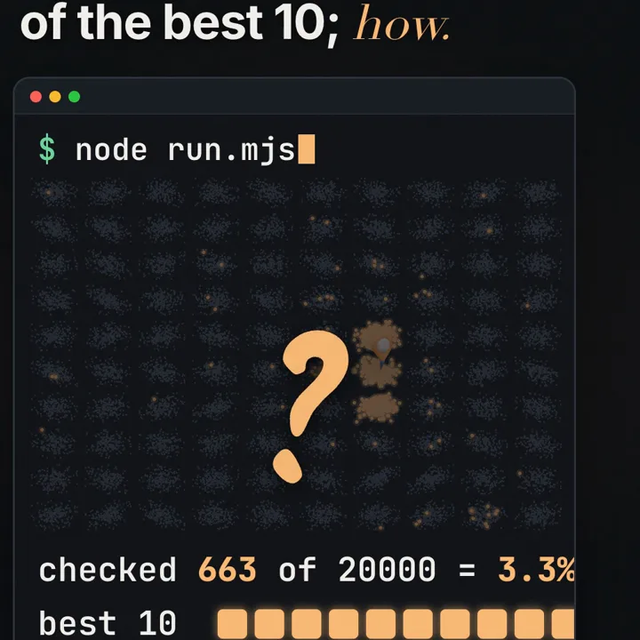
An HNSW index links each vector to a few near neighbours and keeps sparse layers of long links on top, so a search jumps far, then walks close, instead of comparing the query with every vector. In our lab on 20,000 synthetic vectors it touched 776 per query (3.9%), ran a median 7.36x faster than a full scan over 7 runs, and found about 94% of the exact top 10, or 75% at efSearch 10.
| Lab workload | 20,000 synthetic vectors of 64 numbers in 100 clusters, 200 queries, top 10, one M2 Pro, Node 22, single thread. No photos and no embedding model were used |
|---|---|
| Full scan | 20,000 distance evaluations per query, recall 1.000, 2.175 ms average in the canonical run |
| HNSW at efSearch 320 | 776 distinct vectors touched per query (3.9%), 794 distance evaluations, 0.296 ms average, recall@10 0.944 (1,887 of 2,000 true neighbours) |
| Speed spread | 7 back-to-back runs gave 5.0x to 9.9x, median 7.36x. Counts and recall were identical in every run; latency was not |
| The dial | recall@10 rose from 0.750 at efSearch 10 (145 vectors touched) to 0.944 at efSearch 320 (776 touched). The 0.95 target was not reached in the tested range |
| Costs | 2.5 s to build (510 distance evaluations per inserted vector), about 1.61 MB of estimated link payload next to 5.12 MB of float32 vectors |
| Versus a B-tree | Both skip work. A B-tree index returns the same rows as a full scan; HNSW can miss a few true neighbours |
HNSW vector search answers "which stored vectors are closest to this query" without comparing the query with every vector: it walks a layered graph of near-neighbour links and stops once its result list is full and the nearest unexplored candidate is farther than the worst result it holds. The price is that the answer is approximate, and in our lab on 20,000 synthetic vectors the dial that controls it moved recall from 0.750 to 0.944 while the work per query grew from 145 to 776 vectors. Interview version: "Users type 'dog on a beach' into a photo library of millions. Design the search so it does not read every photo."
Prerequisites
Embeddings
An embedding model turns a piece of content into a fixed-length list of numbers so that related content gets nearby vectors. How that works for words and sentences, and why a search for car can find vehicle, is in embeddings explained (AI 11). This article starts where that one stops: you already have the vectors, and the question is how to find the nearest ones fast.
One space for photos and words
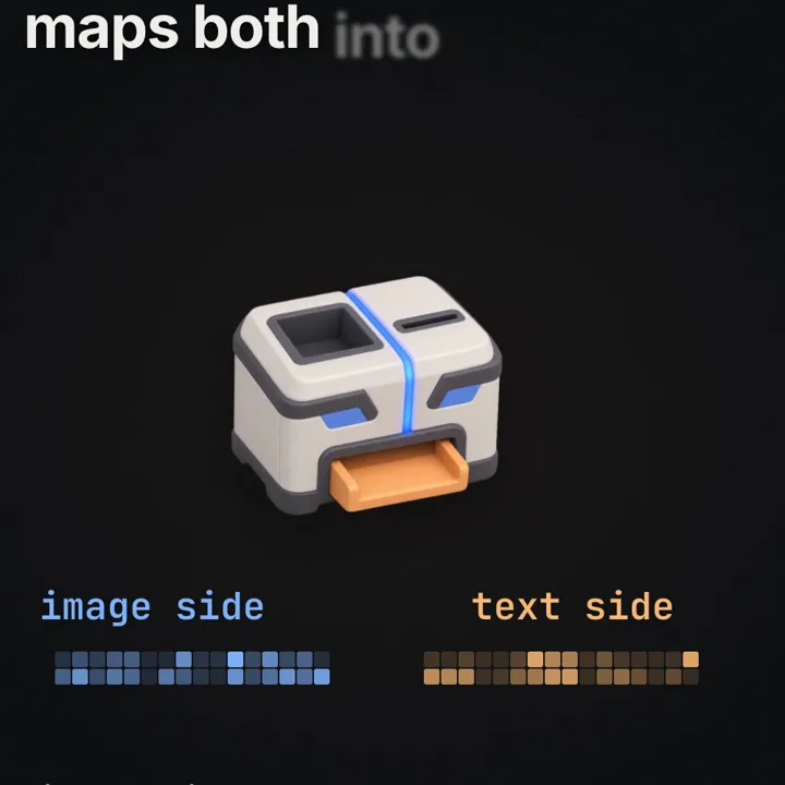
To search photos by a typed sentence, the photo vectors and the sentence vector must be comparable. CLIP (Radford et al., 2021) does this with two encoders, one for images and one for text, trained together on 400 million image and text pairs with a contrastive objective: a matching photo and caption are pushed toward a high cosine similarity, and mismatched pairs in the same batch are pushed apart. After training, "dog on a beach" from the text side lands near photos of dogs on beaches from the image side. Our lab ran no model of any kind. It generated synthetic vectors and measured their search cost and recall.
Distance and cosine
The lab ranks by squared Euclidean distance, ‖q - x‖². For vectors of length 1 (CLIP-style models compare normalized vectors), ‖q - x‖² = 2 - 2·cos(q, x), so sorting by smallest squared distance gives exactly the same order as sorting by largest cosine. Libraries such as Faiss and hnswlib offer both metrics; with normalized vectors the choice changes the numbers, not the ranking.
Definitions
k-nearest-neighbour search (kNN): given a query vector, return the k stored vectors with the smallest distance to it. The lab uses k = 10.
Full scan (flat index): compute the distance from the query to every stored vector and keep the best k. Exact by construction; cost grows with N × d.
Approximate nearest neighbour (ANN) index: a structure that returns most of the true k nearest vectors while computing far fewer distances than a full scan.
HNSW: Hierarchical Navigable Small World graph. Every vector is a node on layer 0 with links to nearby nodes; a random, geometrically shrinking subset also appears on higher layers with links that span longer distances.
M, M0 and efConstruction: build parameters. M is how many links a new node gets per layer (and the cap on upper layers), M0 the cap on layer 0, and efConstruction how wide the search is that finds those links. The lab uses 12, 24 and 60.
efSearch: the query-time width, the number of best candidates the layer-0 search keeps while exploring. It must be at least k.
Recall@10: of the 10 true nearest vectors from the full scan, how many the index returned, averaged over queries. Over 200 queries that is hits out of 2,000.
Distance evaluation and distinct vector touched: the lab counts both. An evaluation is every distance computed; a vector reached on two layers counts twice. Distinct vectors count each id once per query, and the "3.9%" uses that count.
How does HNSW vector search skip most vectors?
The lab (labs/ai-12/run.mjs) generates 20,000 vectors of 64 numbers in 100 clusters. Each cluster really varies along only 8 hidden directions plus a little noise, because real embeddings are clumpy rather than uniform noise. It draws 200 query vectors from the same distribution (plus 20 untimed warm-up queries), computes the exact top 10 for each by full scan, then builds an HNSW index in plain JavaScript and searches it at six efSearch settings. Seeds are fixed, so the data, the graph, every count and every recall value repeat exactly from run to run.
The full scan is the baseline: 20,000 distances of 64 dimensions each, so 1,280,000 coordinate contributions per query, each requiring subtraction, squaring and accumulation, and recall 1.000.
Layers: how many nodes go up
When a vector is inserted, it draws a top level from an exponentially decaying distribution. The paper's rule, which the lab follows:
level = floor( -ln(U) · mL ),   U uniform in (0, 1],   mL = 1 / ln(M)

P(level >= l) = M^(-l)                         lab: M = 12, mL = 1 / ln 12 = 0.402

nodes reaching level l, 20,000 vectors     expected 20,000 / 12^l     the lab's graph
level >= 1                                 1,667                      1,681
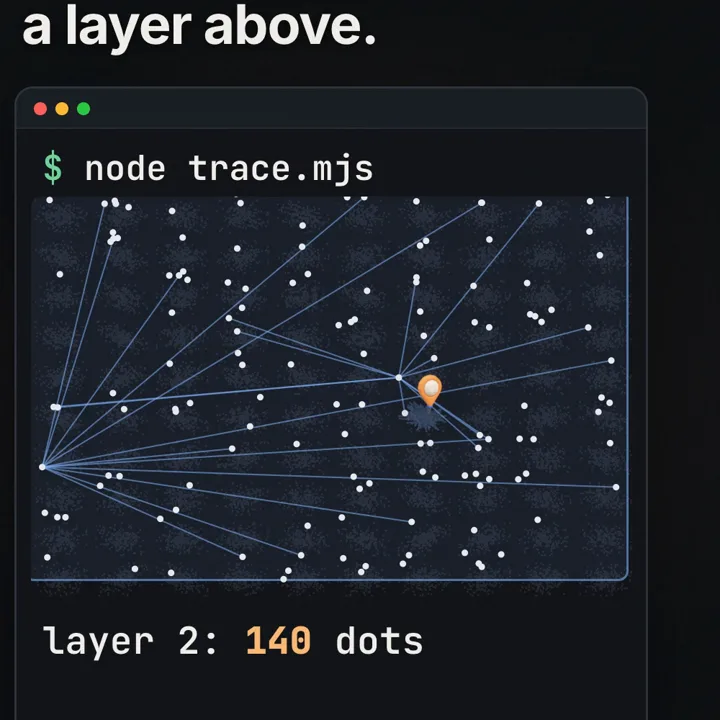
level >= 2                                 139                        140
level >= 3                                 11.6                       6
highest level                              about ln(20,000) / ln(12) = 9.90 / 2.48 = 3.99    3
So 18,319 vectors live only on layer 0, and 6 sit on layer 3. Each layer is about 12 times sparser than the one below, which is what makes the top layers useful: with few nodes, a link between two of them usually crosses a long distance.
Insert: how links are chosen
To insert vector v with level L, the builder starts at the global entry point on the top layer and walks greedily (keep only the single best candidate) down to layer L + 1. From layer L down to 0 it runs a wider search keeping efConstruction = 60 candidates, then picks M = 12 of them as links. The lab uses the paper's heuristic: walk the candidates from closest to farthest and keep one only if it is closer to v than to any neighbour already kept, then top up with the closest skipped ones. That rule spreads links in different directions, and the paper notes it matters most for clustered data, where closest-first linking can leave clusters poorly connected. Every chosen neighbour gets a reverse link to v; if its list goes over the cap (12 upper, M0 = 24 on layer 0), the lab trims it to the closest ones, a simpler step than some libraries use.
Search: jump far, then walk close
A query runs the same two phases:
ep = entry point (the node at the highest level)
for layer = maxLevel down to 1:
    ep = greedy search on this layer from ep with a list of size 1      # jump far
results = beam search on layer 0 from ep with a list of size max(efSearch, k)   # walk close
return the best k of results

beam search keeps two heaps and a visited set:
    candidates   closest first, nodes still to expand
    results      the best ef seen so far, worst on top
start: push (dist(q, ep), ep) into candidates and results, mark ep visited
loop while candidates is not empty: pop the closest candidate c
    if results.size == ef and dist(c) > worst_result_distance: stop
    for each neighbour n of c:
        if n is visited: continue
        mark n visited
        dn = dist(q, n)
        if results.size < ef or dn < worst_result_distance:
            push (dn, n) into candidates and results
            if results.size > ef: remove the worst result
Search stops when the result heap is full and the nearest queued candidate is farther than its worst retained result, or when the queue empties. The rule compares the frontier with what is already held and makes no check that the true nearest vectors are among the results. A larger ef means a longer list to beat and a longer walk. hnswlib's searchBaseLayerST implements the same condition. The paper argues that with the layer structure the number of hops grows roughly with log N for the data it analyses, which is where the logarithmic scaling claims come from. The lab only ran N = 20,000, so it tests none of that scaling.
What does one traced search look like?
labs/ai-12/trace.mjs is run.mjs with logging added. It rebuilds the same index from the same seeds and records search 1 of the 200 (query 0) at efSearch 320 and at 10. It times nothing; all latency figures come from run.mjs.
query 0 belongs to cluster 68 (its exact top 10 are all in cluster 68, which holds 194 vectors)

layer   evaluated   landed on   that node's cluster
3       6           14551       31      (start: entry point 1958, cluster 54)
2       22          3996        68
1       14          11725       68
0       640 at efSearch 320, 98 at efSearch 10

path 1958 -> 14551 -> 3996 -> 11725
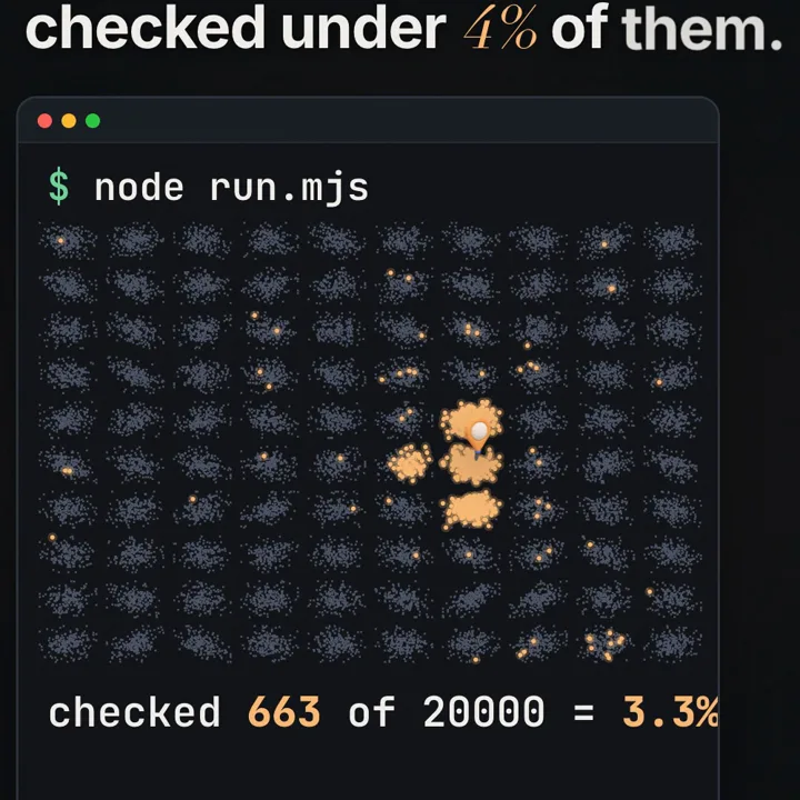
evaluations 6 + 22 + 14 + 640 = 682, distinct vectors 663 (19 repeat evaluations across layers)
efSearch 320: 663 distinct touched, found 10 of 10
efSearch 10:  6 + 22 + 14 + 98 = 140 evaluations, 132 distinct, found 9 of 10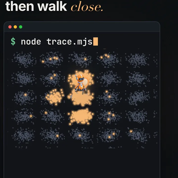
The upper layers cost 42 of the 682 evaluations, about 6%, and by layer 2 the walker was already inside the query's own cluster. Everything after that is layer 0.
At efSearch 10, all 98 layer-0 vectors it evaluated were in cluster 68. It missed one true neighbour (id 13056) and returned id 7416 in its place: the beam was narrow enough to stop before it expanded the node whose links led to 13056.
At efSearch 320, the layer-0 search evaluated all 194 vectors of cluster 68 and 446 vectors from other clusters. The result list had 320 slots and the cluster only has 194 members, so the stop rule could not fire until the beam had pulled in vectors from neighbouring clusters, which are far from the query and cannot be in the top 10. That spill is the extra work you pay for the last few points of recall, and it shows up in the averages below.
Why is 25 times less work only about 7 times faster?
The canonical run is run 5 of 7 (output.txt, results.json):
full scan          2.175 ms average   2.243 ms p95   20,000 evaluations   recall 1.000
HNSW, efSearch 320 0.296 ms average   0.450 ms p95      794 evaluations   776 distinct   recall 0.944

work ratio     20,000 / 794   = 25.2x fewer evaluations
time ratio     2.175 / 0.296  = 7.35x   (the lab prints 7.36 from the unrounded averages)

amortized query time per distance evaluation
  full scan    2.175 ms / 20,000 = 0.109 microseconds
  HNSW         0.296 ms / 794    = 0.373 microseconds   (3.4 times more per evaluation)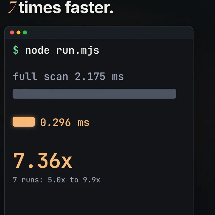
The scan reads one Float32Array front to back, 5.12 MB per query, in a loop the JavaScript JIT compiles tightly, and the access pattern is sequential. The 0.373 microseconds is total HNSW query time divided by evaluations, so it includes everything the walk does besides distance arithmetic. Graph traversal introduces irregular memory access, heap operations and visited checks. These can increase cost per evaluation; this lab does not separate their contributions or measure cache misses. The retained-result heap holds at most ef entries, with O(log ef) operations. The candidate heap can grow beyond ef; its operations cost O(log C), where C is its current size. C++ libraries with SIMD distance code speed up both sides; how the ratio moves there was not tested here.
The run-to-run spread
Seven back-to-back runs on the same Mac (speed-runs.json):
| Run | Full scan avg ms | HNSW ef 320 avg ms | Speedup |
|---|---|---|---|
| 1 | 2.110 | 0.213 | 9.92x |
| 2 | 1.718 | 0.278 | 6.18x |
| 3 | 2.111 | 0.249 | 8.49x |
| 4 | 1.780 | 0.215 | 8.29x |
| 5 (canonical) | 2.175 | 0.296 | 7.36x |
| 6 | 1.530 | 0.306 | 5.00x |
| 7 | 1.639 | 0.268 | 6.11x |
Sorted, the speedups are 5.00, 6.11, 6.18, 7.36, 8.29, 8.49 and 9.92, so the median is 7.36x and run 5 is the median run. The full scan average moved from 1.530 to 2.175 ms (42% apart) and the HNSW average from 0.213 to 0.306 ms (44% apart), and a ratio of two noisy numbers is noisier than either: the 5.00x run paired the fastest scan with the slowest graph search. On a laptop, CPU frequency changes, other apps, JIT decisions and garbage collection all move averages this short. Recall and the evaluation counts never moved, because they depend only on the seeds, so this article leads with work and gives speed as a median with its range. The throughput side of the same problem is in latency vs throughput, measured.
How does efSearch trade recall for speed?
The sweep from the canonical run:
| efSearch | Distinct touched | Evaluations | Share touched | Avg ms (run 5) | p95 ms | Recall@10 |
|---|---|---|---|---|---|---|
| full scan | 20,000 | 20,000 | 100% | 2.175 | 2.243 | 1.000 |
| 10 | 145 | 155 | 0.7% | 0.037 | 0.057 | 0.750 |
| 20 | 181 | 192 | 0.9% | 0.047 | 0.077 | 0.788 |
| 40 | 225 | 237 | 1.1% | 0.064 | 0.101 | 0.823 |
| 80 | 277 | 291 | 1.4% | 0.096 | 0.147 | 0.856 |
| 160 | 331 | 345 | 1.7% | 0.141 | 0.249 | 0.890 |
| 320 | 776 | 794 | 3.9% | 0.296 | 0.450 | 0.944 |
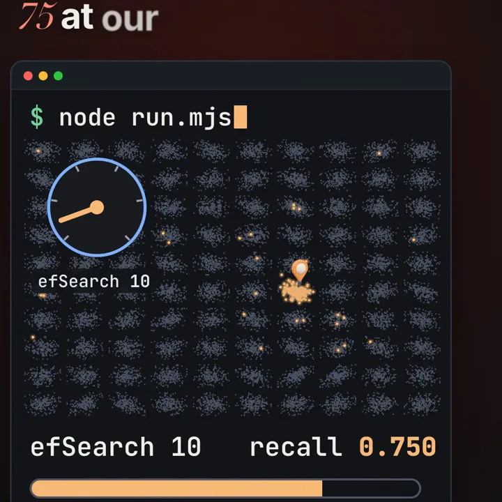
Recall at efSearch 10 is exactly 1,500 of 2,000; at 320 it is 1,887 of 2,000, so 113 true neighbours were still missed across 200 queries. Every doubling from 10 to 160 added roughly 3 to 4 points of recall for 36 to 54 more vectors touched. The last doubling, 160 to 320, added 5.4 points for 445 more vectors, more than double the work. With 100 clusters in 20,000 vectors the average cluster holds 200 vectors, and the trace above showed the mechanism: once ef exceeds the size of the query's cluster, the result list can only fill by reaching into other clusters. The averages are consistent with that spill.
The lab's rule was "pick the lowest efSearch that reaches recall 0.95; if none does, report the best". None did, so the chosen setting is 320 and results.json records "chosen setting reached target recall: 0". Settings above 320, and other values of M or efConstruction, were not tested. The paper and the library documentation describe raising M or efConstruction as the way to build a graph that reaches higher recall, paid for in build time and memory. Whether that would have reached 0.95 here is unknown.
efSearch is a query-time setting in common libraries (hnswlib's set_ef, the efSearch field of Faiss's HNSW index, pgvector's hnsw.ef_search with default 40), so you can tune it without a rebuild. The index cannot report its own misses; recall comes only from comparing with an exact scan, as the lab does.
What does the index cost, and how is it unlike a B-tree?
vectors      20,000 × 64 × 4 bytes                     = 5,120,000 B = 5.12 MB (float32)
links        about 1.61 MB if each stored link is a 4-byte id (estimated, not measured heap)
             1.61 MB / 4 B = about 400,000 links, about 20 per vector
             cap if every list were full: 20,000 × 24 × 4 B = 1.92 MB on layer 0
                                         + 1,827 upper-layer lists × 12 × 4 B = 0.09 MB  -> about 2.01 MB
overhead     1.61 / 5.12 = 31% on top of the vectors

build        2.49 s, 510 distance evaluations per inserted vector
             510 × 20,000 = 10.2 million evaluations = the work of 510 full scans
payback      work: 10,200,000 / (20,000 - 794) = 10,200,000 / 19,206 = about 531 queries
             time (run 5): 2,490 ms / (2.175 - 0.296) ms = 2,490 / 1.879 = about 1,325 queries
The 1,827 upper-layer lists are 1,681 + 140 + 6 from the trace's level counts. The two payback numbers differ for the same reason as the speedup. Real JavaScript heap use is higher than these payload figures and was not measured.
For scale, an assumed library of 1 million photos at 512 dimensions in float32 is 1,000,000 × 512 × 4 = 2.048 GB of vectors, and with the lab's M0 = 24 at most 1,000,000 × 24 × 4 = 96 MB of layer-0 links. That arithmetic is an assumption, not a run. The index is usually kept in RAM; a graph walk that has to fetch random pages from disk pays a disk latency per hop.
Same idea as a B-tree, different guarantee
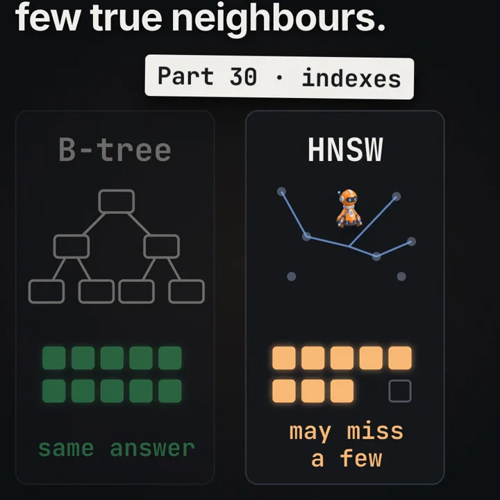
Part 30 of the main series, SQL tuning and indexes, is in the free System Design course. A B-tree index in PostgreSQL works on values with a total order: every key is less than, equal to or greater than every other. Descending from the root page compares the search key with separator keys and rules out whole subtrees with certainty, so a lookup reads a few pages and returns exactly the rows a sequential scan would. The planner may choose either path; the result set is the same.
A B-tree's fixed key order does not generally order vectors by distance to an arbitrary query. Distance to one fixed query would give a sort order, but every query needs a different one, and a stored index has only one. Spatial trees can prune using distance bounds, but that pruning often becomes ineffective as dimensionality grows, so vector search systems use graphs (HNSW), cluster lists (IVF) or compression (product quantization). HNSW's links usually lead to the true neighbours and sometimes do not. The pgvector README puts it from the user's side: queries are exact by default, and adding an HNSW or IVFFlat index makes them approximate, so results can change. The B-tree does less work for the same answer; HNSW does less work and may miss a few.
Worked example
You type "dog on a beach" into a photo library. In a CLIP-style system the text encoder turns it into a vector, and every photo was turned into a vector by the image encoder when it was uploaded. The lab replaces both with synthetic vectors and measures only the search:
library (lab)       20,000 vectors × 64 dims = 5.12 MB float32, 100 clusters
full scan           20,000 evaluations, 1,280,000 coordinate contributions, 2.175 ms (run 5), recall 1.000
HNSW efSearch 320   776 distinct (776 / 20,000 = 3.88%, so 96.1% skipped), 794 evaluations
                    0.296 ms (run 5), recall = 1,887 / 2,000 = 0.9435, rounded to 0.944
speedup             7.36x from unrounded timings in run 5; displayed timings give 2.175 / 0.296 ≈ 7.35x
                    5.0x to 9.9x over 7 runs, median 7.36x
HNSW efSearch 10    145 distinct, 155 evaluations, 0.037 ms (run 5), recall 0.750 = 1,500 / 2,000
one traced search   path 1958 -> 14551 -> 3996 -> 11725; 663 distinct at ef 320 (10 of 10),
                    132 distinct at ef 10 (9 of 10)
costs               2.49 s build, about 1.61 MB links next to 5.12 MB vectors
assumption          everything above is synthetic data on one Mac, not a real photo model
Code
First, the whole idea in a small file you can run anywhere: an exact full scan, a single-layer neighbour graph (HNSW's layer 0 without the upper layers), the same beam search with an ef dial, and a crude "top layer" of 40 random vectors used to pick a starting point. It counts evaluations and recall the same way the lab does.
# graph_search.py  ·  python3 graph_search.py   (Python 3.8+, no packages)
# Exact top-k by full scan vs a greedy beam search on a neighbour graph (HNSW's bottom layer, no upper layers).
import heapq, random

random.seed(7)
N, D, CLUSTERS, K, LINKS = 1000, 16, 20, 10, 4

# Clustered synthetic vectors: a random centre per cluster plus noise (no model, no photos).
centres = [[random.gauss(0, 2) for _ in range(D)] for _ in range(CLUSTERS)]
def point():
    c = random.choice(centres)
    return [x + random.gauss(0, 1.5) for x in c]
data = [point() for _ in range(N)]
queries = [point() for _ in range(50)]

evals = 0
def dist(a, b):                      # squared L2, counted like the lab counts it
    global evals
    evals += 1
    return sum((x - y) ** 2 for x, y in zip(a, b))

def exact_top_k(q):                  # full scan: N distance evaluations, always right
    return [i for _, i in heapq.nsmallest(K, ((dist(q, v), i) for i, v in enumerate(data)))]

# Build: link every vector to its LINKS nearest (by full scan, fine for 1,000 vectors), both directions.
graph = [set() for _ in range(N)]
for i, v in enumerate(data):
    for _, j in heapq.nsmallest(LINKS + 1, ((dist(v, w), j) for j, w in enumerate(data))):
        if j != i:
            graph[i].add(j); graph[j].add(i)

def beam_search(q, ef, start=0):     # the layer-0 loop of HNSW: a candidate heap and a result heap of size ef
    seen = {start}
    d0 = dist(q, data[start])
    cand, best = [(d0, start)], [(-d0, start)]
    while cand:
        d, c = heapq.heappop(cand)
        if len(best) >= ef and d > -best[0][0]:
            break                    # the closest unexplored candidate is worse than the worst kept result
        for n in graph[c]:
            if n in seen:
                continue
            seen.add(n)
            dn = dist(q, data[n])
            if len(best) < ef or dn < -best[0][0]:
                heapq.heappush(cand, (dn, n)); heapq.heappush(best, (-dn, n))
                if len(best) > ef:
                    heapq.heappop(best)
    return [i for _, i in sorted((-d, i) for d, i in best)][:K]

# A crude "top layer": 40 random vectors. Jump far = pick the closest of them, then walk close from there.
top = random.sample(range(N), 40)
def jump_then_walk(q, ef):
    entry = min(top, key=lambda i: dist(q, data[i]))
    return beam_search(q, ef, start=entry)

truth = [exact_top_k(q) for q in queries]
print(f"full scan: {N} evaluations per query, recall@{K} 1.000")
for name, search in (("walk only from vector 0", beam_search), ("jump far, then walk", jump_then_walk)):
    for ef in (10, 20, 40, 80):
        evals = 0
        hits = sum(len(set(search(q, ef)) & set(t)) for q, t in zip(queries, truth))
        print(f"{name:24} ef {ef:2}: {evals / len(queries):4.0f} evaluations/query, "
              f"recall@{K} {hits / (K * len(queries)):.3f}")
What to observe: it runs in a few seconds and prints the same lines every time (fixed seed). On our machine the walk from a fixed start needed ef 80 and 225 evaluations per query to reach recall 0.896, because it often begins in the wrong cluster and has to cross the graph. With the crude top layer it reached 0.900 at ef 10 for 86 evaluations (40 of them spent choosing the entry) and 0.986 at ef 40 for 121. Raise LINKS to 6 and the fixed-start walk improves too, because more links connect the clusters better; set the noise down to 0.6 and the clusters become islands: in our tries the walk from vector 0 then stayed near recall 0.04 at every ef.
Second, the full lab, which needs Node.js 22 or later and no packages:
# from the repo root
node labs/ai-12/run.mjs      # data, index build, full scan, efSearch sweep; last line is RESULT {...}
node labs/ai-12/trace.mjs    # same seeds and index; records search 1 of 200 and rewrites labs/ai-12/trace.json
What to observe in run.mjs: the distinct-touched column (145 to 776), the recall column (0.750 to 0.944) and the conclusion line, which is built from the measured numbers and would say so if HNSW were not faster on your machine. Counts and recall should match this article exactly; milliseconds will not. The run has a 50 second deadline and prints INCOMPLETE rather than a partial result if it hits it.
Failure modes and edge cases
- Returning k results does not establish recall. Monitor returned-result count separately from recall against exact ground truth. Filters, too few eligible rows, disconnected parts of the graph and scan limits can all leave fewer than k results, and pgvector's iterative index scans still stop at their configured limits (
hnsw.max_scan_tuples). After every rebuild, parameter change or large data change, run sample queries through an exact scan, compare, and alert on a drop in either number. Compare approximate and exact queries with identical filters in the same repeatable-read transaction. For the exact query, useSET LOCAL enable_indexscan = offand verify the plan withEXPLAIN(pgvector's monitoring notes use the same setting). If fewer than k eligible rows exist, calculate recall against the available exact results and report result count separately. - On clustered data a bad entry point hurts. The Python demo shows a walk stuck in the wrong cluster. Upper layers and the diverse-link heuristic reduce this, but poorly connected clusters still show up as single queries with near-zero recall while the mean looks fine. Watch the per-query recall distribution.
- Deletion behavior depends on the implementation. hnswlib marks nodes deleted (
mark_deleted) and excludes them from results while retaining them for traversal. pgvector repairs graph links during VACUUM before marking elements deleted. Measure recall, traversal cost and index size under representative churn, and rebuild when those numbers warrant it. - Filters shrink results. "Dogs on a beach from last summer" adds a filter, and filtering after the ANN step shrinks the result: pgvector's README notes that with
hnsw.ef_search40 and a filter matching 10% of rows, about 4 rows survive. Use iterative index scans, a larger ef, partitioning or a partial index. - The lab's queries come from the same distribution as the stored vectors. Text query vectors can sit in different regions of a CLIP-style space from image vectors, so image-to-image recall can overstate text-to-image recall. Evaluate with queries users actually type.
- A new embedding model changes every vector. Store the model id with each vector, build the new index beside the old one, and switch reads after checking recall.
- Benchmarks on a laptop are noisy: one run said 9.9x and another 5.0x. Report medians and ranges, warm up first, and lead with evaluations per query, which do not depend on the machine.
Trade-offs
| Option | Good for | Costs you | Use when |
|---|---|---|---|
| Full scan (flat) | Exact answers, no build, trivial updates | N × d per query: 20,000 evaluations in the lab | Small sets, ground truth for recall checks, or batch jobs |
| HNSW | High recall at a small fraction of the work (776 of 20,000 at 0.944) | Build time (2.5 s in the lab), link memory (about 31% here), harder deletes, misses | Read-heavy search that fits in RAM |
| HNSW with low efSearch | Lowest latency (145 touched, 0.037 ms in run 5) | Recall 0.750 in the lab | When measured candidate recall meets the application's target |
| IVF (cluster lists) | Fast build, small overhead | Recall depends on how many lists you probe; clusters drift and need retraining | Very large sets, frequent rebuilds |
| IVF with product quantization | Much smaller memory | Approximate distances, lower recall without reranking | Sets too large for full-precision vectors in RAM |
| B-tree on a scalar column | Exact range and equality lookups | Not applicable to nearest-vector search | Filters such as date or owner next to the vector search |
For reranking, retrieve R candidates where R exceeds the final k, and measure candidate recall against the exact top-k before choosing efSearch. A reranker can reorder only the retrieved candidates. If the vectors are stored at full precision and the reranker uses the same distance, sorting the returned candidates again changes nothing; a reranker earns its place when it scores with something the index did not, such as full-precision vectors after a quantized index or a cross-encoder model.
Common mistakes
In an interview
Start by asking how many photos there are, how often they change, the query rate and latency target, whether results need filters such as owner or date, and whether missing a few results is acceptable. State your assumptions out loud, for example 1 million photos, 512-dimension vectors and p95 under 100 ms. The design is an image encoder at upload time, a text encoder at query time, vectors in an HNSW index in RAM, and filters applied together with the index; if a reranker follows, retrieve more candidates than the final k and size efSearch by candidate recall. For the deep part, explain layers and links, the upper-layer descent and layer-0 beam search, the stop rule, and memory as N × d × 4 bytes plus links. The trade-offs to name are recall against latency through efSearch, build time and memory through M and efConstruction, and HNSW against IVF with quantization at larger scale. Close with how you would operate it: recall measured against an exact scan on sampled queries, returned-result counts watched separately, latency reported as a median with range, and a maintenance plan for deletes and model changes.
A model with an image side and a text side, trained together like CLIP, turns each photo and each typed query into vectors in one space, so search becomes finding the nearest photo vectors. A full scan compares the query with every vector and is exact, but its cost grows with every photo. I would put the vectors in an HNSW index: every vector links to a few near neighbours, and a sparse set of upper layers holds long links, so a query jumps far on the top layers, then runs a beam search on the bottom one that stops when its result list is full and the nearest queued candidate is farther than the worst result it holds, or when the queue empties. In a small lab on 20,000 synthetic vectors that touched 776 vectors per query, about 4%, and was a median 7.36 times faster than a full scan across seven runs, with recall 0.944. It is approximate, unlike a B-tree index, so I would tune efSearch on a recall curve, measure recall against an exact scan on sample queries, and plan for filters, deletes and model changes.
Practice
BeginnerWhy does ranking by squared distance give the same order as cosine for unit vectors?
For length-1 vectors, ‖q - x‖² = 2 - 2·cos(q, x). The smallest distance is always the largest cosine.
BeginnerWhat share of the 20,000 vectors did HNSW touch at efSearch 320, and how many did it skip?
776 distinct vectors per query on average, 3.88%, so about 96.1% were never compared.
IntermediateWith M = 12, how many of 20,000 nodes should reach level 2, and how many did?
P(level ≥ 2) = 12^(-2), so 20,000 / 144 = 139 expected; the lab's graph had 140.
IntermediateWhen does the layer-0 beam search stop?
When its result list holds ef entries and the closest unexplored candidate is farther than the worst of them, or when the candidate queue empties. A larger ef means a longer list to beat, so a longer walk.
IntermediateWhy did 7 runs of the same deterministic lab give 5.0x to 9.9x?
Counts and recall depend only on the seeds; latency depends on CPU frequency, other processes, JIT and garbage collection. The speedup is a ratio of two noisy averages, so it is noisier than either. Median 7.36x.
Advanced794 evaluations against 20,000 is 25.2x less work. Why only 7.36x less time?
The amortized query time per distance evaluation was about 0.373 microseconds for HNSW against 0.109 for the scan. Graph traversal adds irregular memory access, heap operations and visited checks; the lab did not separate their contributions or measure cache misses.
AdvancedGoing from efSearch 160 to 320 added 445 touched vectors for 5.4 points of recall. What explains the jump?
Clusters average 200 vectors. Once the result list is bigger than the query's cluster, it can only fill from neighbouring clusters. The trace shows it: at 320, all 194 vectors of cluster 68 plus 446 from other clusters.
AdvancedHow many queries does the lab's index build take to pay back?
In evaluations, 10.2 million / (20,000 - 794) ≈ 531 queries. In run-5 time, 2,490 ms / 1.879 ms ≈ 1,325 queries, higher because graph evaluations cost more.
Cheat sheet
| Term or formula | Meaning |
|---|---|
| Full scan cost | N × d coordinate contributions per query; 20,000 × 64 = 1.28 million in the lab |
| Vector memory | N × d × 4 bytes; 5.12 MB in the lab |
| Link memory (estimate) | stored links × 4 bytes; about 1.61 MB in the lab |
| Level rule | floor(-ln U · mL), mL = 1/ln M; P(level ≥ l) = M^(-l) |
| M, M0 | Links per new node and per upper-layer list; cap on layer 0 (12 and 24 in the lab) |
| efConstruction | Build-time search width; 60 in the lab |
| efSearch | Query-time result list size, at least k; the recall dial |
| Stop rule | Result list full and closest queued candidate farther than worst kept result, or queue empty |
| Recall@10 | True top-10 found / 10, averaged; 0.750 at ef 10, 0.944 at ef 320 |
| Distance evaluations vs distinct touched | Every distance computed vs each id once per query (794 vs 776) |
| Unit-vector identity | ‖q - x‖² = 2 - 2·cos(q, x) |
| B-tree vs HNSW | Same answer as a scan vs may miss a few |
Further reading
- Malkov and Yashunin give the HNSW insert and search algorithms, the level distribution, the neighbour-selection heuristic and the origin of M and ef.
- Radford et al. (CLIP) show how an image encoder and a text encoder are trained together into one embedding space.
- The Faiss indexes page lists exact flat indexes next to HNSW, IVF and product quantization, with their parameters.
- hnswlib is a widely used HNSW implementation; its header
hnswalg.hholds the search loop and the mark-deleted logic. - pgvector covers HNSW and IVFFlat inside PostgreSQL, exact versus approximate results, filtering and iterative scans.
- ANN-Benchmarks describes how to compare ANN libraries on recall against queries per second.
Related in this series: the retrieval loop that uses these indexes is in how AI finds one line in 100 pages (AI 4), and sizing a search tier under load uses the arithmetic in performance vs scalability, measured.
This article describes general patterns and our own small lab on synthetic vectors with a teaching HNSW in JavaScript on one Mac. No photos, no embedding model and no production library were run. The numbers are not a benchmark of any model, library, database or product, and nothing here describes any company's private systems.
Frequently asked questions
How does HNSW skip most of the vectors?
It stores a graph: each vector links to a few near neighbours, and a few vectors also sit on sparse upper layers with long links. A search starts at the top, hops toward the query, drops down, and on the bottom layer explores only the neighbourhood around the best candidates. In our lab that meant 776 of 20,000 vectors per query at efSearch 320.
Is HNSW search exact?
No. It is approximate. In our lab it found 1,887 of the 2,000 true top-10 neighbours at efSearch 320 (recall 0.944) and 1,500 of 2,000 at efSearch 10. A full scan always finds all of them.
What does efSearch do?
It is the size of the result list the bottom-layer search keeps while it explores. A larger value explores more of the graph, which raises recall and costs more distance evaluations and time. In the lab, 10 gave 0.750 recall at 145 vectors touched and 320 gave 0.944 at 776.
Why was the speedup 7.36x and not 25x?
HNSW did about 25 times fewer distance evaluations (794 against 20,000), but each one cost more. In run 5 the amortized query time per distance evaluation was about 0.373 microseconds against 0.109 for the scan. Graph traversal adds irregular memory access, heap operations and visited checks; the lab did not separate their contributions or measure cache misses.
Does this lab say how fast a real photo search is?
No. The vectors are synthetic, no model ran, the index is a teaching version in JavaScript, and it holds 20,000 vectors. It shows the shape of the trade-off, not production numbers for any library or product.
How is an HNSW index different from a B-tree index?
A B-tree orders keys on one sortable value, so an index lookup returns exactly the rows a full scan would. A B-tree's fixed key order does not generally order vectors by distance to an arbitrary query, and spatial trees that prune with distance bounds lose most of that pruning as dimensions grow, so HNSW uses a graph walk that usually, but not always, reaches the true nearest vectors.
Sources
- Malkov and Yashunin, Efficient and robust approximate nearest neighbor search using Hierarchical Navigable Small World graphs (arXiv 1603.09320)arxiv.org
- Radford et al., Learning Transferable Visual Models From Natural Language Supervision (CLIP, arXiv 2103.00020)arxiv.org
- Faiss wiki: Faiss indexesgithub.com
- hnswlib: header-only C++/Python library for fast approximate nearest neighborsgithub.com
- pgvector: open-source vector similarity search for Postgresgithub.com
- Aumüller, Bernhardsson and Faithfull, ANN-Benchmarks: A Benchmarking Tool for Approximate Nearest Neighbor Algorithms (arXiv 1807.05614)arxiv.org

Written by a software engineer and system architect with 10+ years of building production web, payment, ticketing and accounting systems in Japan and Nepal. About us